Collision Warning Using 2-D Lidar

This example uses:

This example shows how to detect obstacles and warn of possible collisions using 2-D lidar data.

Overview

Logistics warehouses are increasingly mounting 2-D lidars on automatic guided vehicles (AGV) for navigation purposes, due to the affordability, long range, and high resolution of the sensor. The sensors assist in collision detection, which is an important task for the safe navigation of AGVs in complex environments. This example shows how to represent a robot workspace populated with obstacles, generate 2-D lidar data, detect obstacles, and provide a warning before an impending collision.

Create a Warehouse Map

To represent the environment of the robot workspace, define a binaryOccupancyMap (Navigation Toolbox) object that contains the floor plan of the warehouse. Each cell in the occupancy grid has a logical value. An occupied location is represented as 1 and a free location is represented as 0. You can use the occupancy information to generate synthetic 2-D lidar data.

Add obstacles to the map near to the defined route of AGV.

% Create a binary warehouse map and place obstacles at defined locations
map = helperCreateBinaryOccupancyMap;

% Visualize map with obstacles and AGV
figure
show(map)
title('Warehouse Floor Plan With Obstacles and AGV')

% Add AGV to the map
pose = [5 40 0];
helperPlotRobot(gca,pose);

Figure contains an axes object. The axes object with title Warehouse Floor Plan With Obstacles and AGV, xlabel X [meters], ylabel Y [meters] contains 2 objects of type image, patch.

Simulate 2-D Lidar Sensor

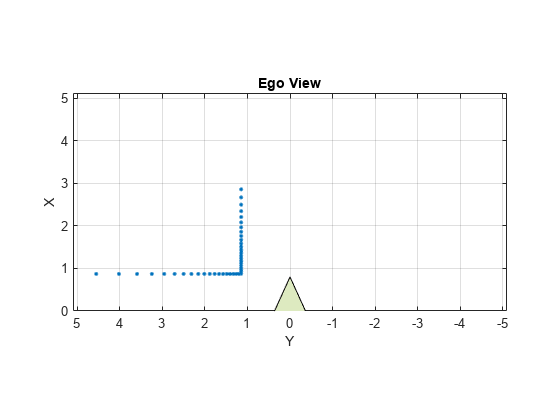
Simulate 2-D lidar sensor using a rangeSensor object to gather lidar readings for the generated map. Load a MAT-file containing the predefined waypoints of the AGV into the workspace. Use the simulated lidar sensor to return range and angle readings for a pose of the AGV, and then use the ranges and angles to generate a lidarScan object that contains the 2-D lidar scan.

% Simulate lidar sensor and set the detection angles to [-pi/2 pi/2]
lidar = rangeSensor;
lidar.HorizontalAngle = [-pi/2 pi/2];

% Set min and max values of the detectable range of the sensor in meters
lidar.Range = [0 5];

% Load waypoints through which AGV moves
load waypoints.mat
traj = waypointsMap;

% Select a waypoint to visualize scan data
Vehiclepose = traj(350,:);

% Generate lidar readings
[ranges,angles] = lidar(Vehiclepose,map);

% Store and visualize 2-D lidar scan
scan = lidarScan(ranges,angles);
plot(scan)
title('Ego View')
helperPlotRobot(gca,[0 0 Vehiclepose(3)]);

Figure contains an axes object. The axes object with title Ego View, xlabel X, ylabel Y contains 2 objects of type line, patch. One or more of the lines displays its values using only markers

Set Up Visualization

Set up a figure window that displays AGV movement in the warehouse, the associated lidar scans of the environment, displays obstacles as filled circles in bird's eye view, and color-coded collision warning messages. The color used for each warning signifies the likelihood of a collision based on the detection area zone that the obstacle occupies at that waypoint.

% Set up display
display = helperVisualizer;

% Plot warehouse map in the display window
hRobot = plotBinaryMap(display,map,pose);

Collision Warning Based on Zones

Collision warnings only appear if an obstacle falls within the detection area of the AGV.

Define the Detection Area

Create a custom detectable area with different colors, shapes, and modify the area of color regions on figure GUI. Run the below portion of code and modify the polygon handles to accommodate your requirements of the detection area. The code below creates 3 polygon handles of semi-circular regions with a radius of 5, 2, 1 in meters and AGV is positioned at [0 0]. Modify the radius or change the polygon objects to create a custom detection area.

figure
detAxes = gca;
title(detAxes,'Define Detection Area')
axis(detAxes,[-2 10 -2 4])
xlabel(detAxes,'X')
ylabel(detAxes,'Y')
axis(detAxes,'equal')
grid(detAxes,'minor')
t = linspace(-pi/2,pi/2,30)';

% Specify color values - white, yellow, orange, red
colors = [1 1 1; 1 1 0; 1 0.5 0; 1 0 0];

% Specify radius in meters
radius = [5 2 1];

% Create a 3x1 matrix of type Polygon
detAreaHandles = repmat(images.roi.Polygon,[3 1]);

pos = [cos(t) sin(t)]*radius(1);
pos = [0 -2; pos(14:17,:); 0 2];
detAreaHandles(1) = drawpolygon( ...
	'Parent',detAxes, ...
	'InteractionsAllowed','reshape', ...
	'Position',pos, ...
	'StripeColor','black', ...
	'Color',colors(2,:));

pos = [cos(t) sin(t)]*radius(2);
pos = [0 -1.5; pos(12:19,:); 0 1.5];
detAreaHandles(2) = drawpolygon( ...
	'Parent',detAxes, ...
	'InteractionsAllowed','reshape', ...
	'Position',pos, ...
	'StripeColor','black', ...
	'Color',colors(3,:));

pos = [cos(t) sin(t)]*radius(3);
pos = [0 -1; pos(10:21,:); 0 1];
detAreaHandles(3) = drawpolygon( ...
    'Parent',detAxes, ...
	'InteractionsAllowed','reshape', ...
	'Position',pos, ...
	'StripeColor','black', ...
	'Color',colors(4,:));

% Pausing for the detection area window to load
pause(2)

To save the created detection area, run the helperSaveDetectionArea function. Use the axes handle of the figure with the detection area polygons and the associated detAreaHandles variable as input arguments. The function outputs the detection area, as a matrix of datatype uint8, and a bounding box. The blue rectangle around the detection area represents the bounding box.

% Axes of the figure window containing the polygon handles
axesDet = gca; 
[detArea,bbox] = helperSaveDetectionArea(axesDet,detAreaHandles);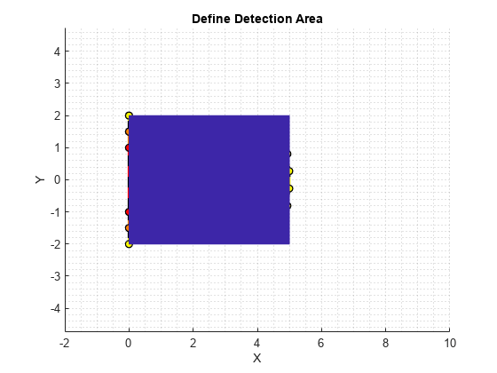

Figure contains an axes object. The axes object with title Define Detection Area, xlabel X, ylabel Y contains 4 objects of type images.roi.polygon, image.

% Make detection area transparent by scaling colors
% alphadata = double(detArea ~= 0)*0.5;
ax3 = getDetectionAreaAxes(display);
h = imagesc(ax3, [bbox(1) (bbox(1)+bbox(3))], ...
    -[bbox(2) (bbox(2)+bbox(4))], ...
    detArea);

colormap(ax3,colors);

% Plot detection area
plotObstacleDisplay(display)

Run Simulation

The detection area is divided into three levels as: red, orange, and yellow. Each region is associated with a specific degree of danger:

Red — Collision is imminent
Orange — High chance of collision
Yellow — Apply caution measures

Obstacles that do not fall within the detection range are at safe distance from AGV. These are the primary steps involved in collision warning:

Simulate 2-D lidar and extract point cloud data.
Segment point cloud data into obstacle clusters.
Loop over each obstacle to check for possible collisions.
Issue a warning based on the danger level of obstacles.
Display obstacles close to the AGV.

% Move AGV through waypoints
for ij = 27:size(traj,1)
    currentPose = traj(ij,:);

Simulate 2-D Lidar and Extract Point Cloud Data

Gather lidar readings of the map using the simulated sensor. Load the current pose of the AGV from the waypoints file. Use the rangeSensor object you created to get range and angle measurement.

    % Retrieve lidar scans
    [ranges,angles] = lidar(currentPose,map);
    scan = lidarScan(ranges,angles);
    
    % Store 2-D scan as point cloud
    cart = scan.Cartesian;
    cart(:,3) = 0;
    pc = pointCloud(cart);

Segment Point Cloud Data into Obstacle Clusters

Use the pcsegdist function to segment the scanned point cloud into clusters, using minimum euclidean distance between the points as the segmentation criterion.

    % Segment point cloud into clusters based on euclidean distance
    minDistance = 0.9;
    [labels,numClusters] = pcsegdist(pc,minDistance);

Update Visualization Window with Map and Scan Data

    % Update display map
    updateMapDisplay(display,hRobot,currentPose);
    
    % Plot 2-D lidar scans
    plotLidarScan(display,scan,currentPose(3));
    
    % Delete obstacles from last scan to plot next scan line
    if exist('sc','var')
        delete(sc)
        clear sc
    end

Loop Over Each Obstacle to Find the Likelihood of Collisions

Loop through the clusters based on their labels, to extract the points located inside them.

    nearxy = zeros(numClusters,2);
    maxlevel = -inf;
    % Loop through all the clusters in pc
    for i = 1:numClusters
        c = find(labels == i);
        % XY coordinate extraction of obstacle
        xy = pc.Location(c,1:2);

Convert the world position of each obstacle into the camera coordinate system.

        % Convert to normalized coordinate system (0-> minimum location of detection
        % area, 1->maximum position of detection area)
        a = [xy(:,1) xy(:,2)] - repmat(bbox([1 2]),[size(xy,1) 1]);
        b = repmat(bbox([3 4]),[size(xy,1) 1]);
        xy_org = a./b;

        % Coordinate system (0, 0)->(0, 0), (1, 1)->(width, height) of detArea
        idx = floor(xy_org.*repmat([size(detArea,2) size(detArea,1)],[size(xy_org,1) 1]));

Extract the indices of obstacle points that lie in the detection area.

        % Extracts as an index only the coordinates in detArea
        validIdx = 1 <= idx(:,1) & 1 <= idx(:,2) & ...
            idx(:,1) <= size(detArea,2) & idx(:,2) <= size(detArea,1);

For each valid obstacle point, find the associated value in the detection matrix. The maximum value of all associated points in the detection matrix determines the level of danger represented by that obstacle. Display a colored circle based on the danger level of the obstacle in the Warning Color pane of the visualization window.

        % Round the index and get the level of each obstacle from detArea
        cols = idx(validIdx,1);
        rows = idx(validIdx,2);
        levels = double(detArea(sub2ind(size(detArea),rows,cols)));

        if ~isempty(levels)
            level = max(levels);
            maxlevel = max(maxlevel,level);
            xyInds = find(validIdx);
            xyInds = xyInds(levels == level);
            
            % Get the nearest coordinates of obstacle in detection area
            nearxy(i,:) = helperNearObstacles(xy(xyInds,:));
        else
            % Get the nearest coordinates of obstacle in the cluster
            nearxy(i,:) = helperNearObstacles(xy);
        end
    end
    % Display a warning color representing the danger level. If the
    % obstacle does not fall in the detection area, do not display a color.
    switch maxlevel
        % Red region
        case 3
            circleDisplay(display,colors(4,:))
        % Orange region
        case 2
            circleDisplay(display,colors(3,:))
        % Yellow region
        case 1
            circleDisplay(display,colors(2,:))
        % Default case
        otherwise
            circleDisplay(display,[])
    end

Display Points of Obstacles Closest to the AGV

As most of the obstacles in the warehouse are linear and long, display only the point of each obstacle cluster closest to the AGV. Obstacles display as filled circles in the Bird's-Eye Plot pane of the visualization window.

    for i = 1:numClusters
        % Display obstacles if exist in the mentioned range of axes3
        sc(i,:) = displayObstacles(display,nearxy(i,:));
    end
    updateDisplay(display)
    pause(0.01)
end

Supporting Files

helperCreateBinaryOccupancyMap creates a warehouse map of the robot workspace

function map = helperCreateBinaryOccupancyMap()
% helperCreateBinaryOccupancyMap Creates a warehouse map with specific
% resolution passed as arguments to binaryOccupancyMap

map = binaryOccupancyMap(100,80,1);
occ = zeros(80,100);
occ(1,:) = 1;
occ(end,:) = 1;
occ([1:30,51:80],1) = 1;
occ([1:30,51:80],end) = 1;
occ(40,20:80) = 1;
occ(28:52,[20:21 32:33 44:45 56:57 68:69 80:81]) = 1;
occ(1:12,[20:21 32:33 44:45 56:57 68:69 80:81]) = 1;
occ(end-12:end,[20:21 32:33 44:45 56:57 68:69 80:81]) = 1;

% Set occupancy value of locations
setOccupancy(map,occ);

% Add obstacles to the map at specific locations. Inputs to
% helperAddObstacle are obstacleWidth, obstacleHeight and obstacleLocation.
helperAddObstacle(map,5,5,[10,30]);
helperAddObstacle(map,5,5,[20,17]);
helperAddObstacle(map,5,5,[40,17]);
end

%helperAddObstacle Adds obstacles to the occupancy map
function helperAddObstacle(map,obstacleWidth,obstacleHeight,obstacleLocation)
values = ones(obstacleHeight,obstacleWidth);
setOccupancy(map,obstacleLocation,values)
end