Combine Dissimilar Grids by Converting Regular Grid to Geolocated Data Grid
This example shows how to combine an elevation data grid and an attribute (color) data grid that cover the same region but are gridded differently. The example drapes slope data from a regular data grid on top of elevation data from a geolocated data grid. The example uses the geolocated data grid as the source for surface elevations and transforms the regular data grid into slope values, which are then sampled to conform to the geolocated data grid (creating a set of slope values for the diamond-shaped grid) and color-coded for surface display. This approach works with any dissimilar grids, although the two data sets in this example actually have the same origin (the geolocated grid derives from the topo60c data set).
Load the geolocated data grid from the mapmtx file and the regular data grid from the topo60c file. The mapmtx file actually contains two regions but this example only uses the diamond-shaped portion, lt1, lg1, and map1, centered on the Middle East.
load mapmtx lt1 lg1 map1
load topo60c
Compute the surface aspect, slope, and gradients for topo60c. This example only uses the slopes in subsequent steps.
[aspect,slope,gradN,gradE] = gradientm(topo60c,topo60cR);
Use the geointerp function to interpolate slope values to the geolocated grid specified by lt1 and lg1. The output is a 50-by-50 grid of elevations matching the coverage of the map1 variable.
slope1 = geointerp(slope,topo60cR,lt1,lg1);
Set up a figure with a Miller projection and use surfm to display the slope data. Specify the z -values for the surface explicitly as the map1 data, which is terrain elevation. The map mainly depicts steep cliffs, which represent mountains (the Himalayas in the northeast), and continental shelves and trenches.
figure
axesm miller
surfm(lt1,lg1,slope1,map1)
The coloration depicts steepness of slope. Change the colormap to make the steepest slopes magenta, the gentler slopes dark blue, and the flat areas light blue:
colormap cool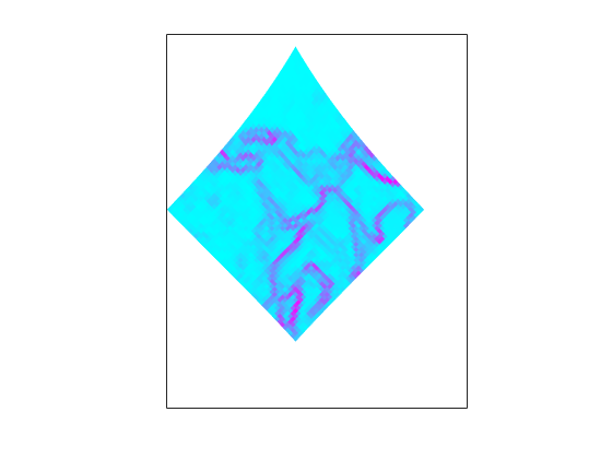
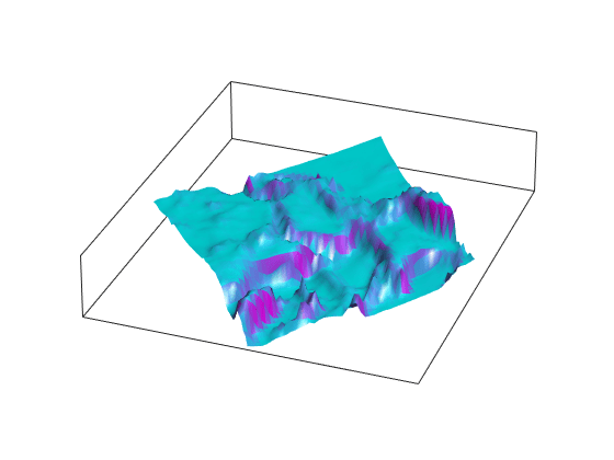
Use view to get a southeast perspective of the surface from a low viewpoint. In 3-D, you can see the topography as well as the slope.
view(20,30)
daspectm('meter',200)
The default rendering uses faceted shading (no smooth interpolation). Make the surface shiny with Gouraud shading and specify lighting from the east (the default of camlight lights surfaces from over the right shoulder of the viewer).
material shiny
camlight
lighting Gouraud
Remove the white space and view the figure in perspective mode.
axis tight
ax = gca;
ax.Projection = 'perspective';