Main Content

los2

Line-of-sight visibility between two points on or above terrain

Description

Specify Coordinates and Heights

vis = los2(Z,R,lat1,lon1,lat2,lon2) determines whether the point specified by lat1 and lon1 has line-of-sight visibility with the point specified by lat2 and lon2. Specify spatially referenced terrain data, in meters, using Z and R. This function assumes that the Earth is a sphere.

vis = los2(Z,R,lat1,lon1,lat2,lon2,h1) specifies the height, in meters, of the first point.

example

vis = los2(Z,R,lat1,lon1,lat2,lon2,h1,h2) specifies the height, in meters, of the second point.

vis = los2(Z,R,lat1,lon1,lat2,lon2,h1,h2,h1ref) references the height of the first point to either the terrain (ground level) or the sphere (mean sea level).

vis = los2(Z,R,lat1,lon1,lat2,lon2,h1,h2,h1ref,h2ref) references the height of the second point to either the terrain (ground level) or the sphere (mean sea level).

Specify Reference Sphere

vis = los2(Z,R,lat1,lon1,lat2,lon2,h1,h2,h1ref,h2ref,rad) specifies the radius in meters of the reference sphere. This syntax is useful for finding line-of-sight visibility for planetary bodies other than Earth.

vis = los2(Z,R,lat1,lon1,lat2,lon2,h1,h2,h1ref,h2ref,rad,effectiveRad) specifies a larger radius for the propagation of line-of-sight paths. You can use this syntax to account for the curvature of signal paths due to refraction in the atmosphere.

Query Intermediate Points

[vis,visprofile,dist,h,lattrk,lontrk] = los2(___) determines line-of-sight visibility for intermediate points between the first and second points, using any combination of input arguments from the previous syntaxes. For each intermediate point, the function returns the visibility in visprofile, the distance from the first point in dist, the height in h, the latitude in lattrk, and the longitude in lontrk. The number of intermediate points depends on the resolution of the terrain data.

example

Display and Interactively Select Coordinates

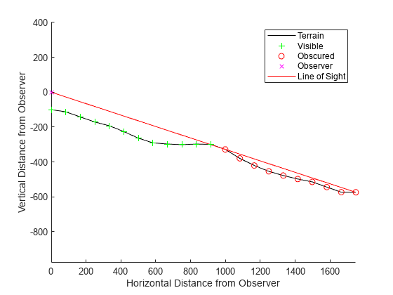
los2(___) displays the visibility profile between the two points in a new figure on Cartesian axes. The figure illustrates the terrain, the observer, the line of sight, the visible points, and the obstructed points.

example

[___] = los2 enables you to interactively select two points on the current axesm-based map and then determines whether the points have line-of-sight visibility, returning any combination of output arguments from previous syntaxes. If the current object on the map is a surface, then the function uses the z-coordinate data (the ZData property) as the terrain elevation data. Otherwise, the function uses z-coordinate data from the first surface it finds on the map. If the surface does not have z-coordinate data, then the function uses the color data (the CData property), instead.
Examples

collapse all

Determine whether two points have line-of-sight visibility. Then, display the visibility profile.

Read terrain data for an area around South Boulder Peak into the workspace as an array and a reference object. Prepare the data for analysis by specifying the output type as "double".

[Z,R] = readgeoraster("n39_w106_3arc_v2.dt1","OutputType","double");

Specify the coordinates of South Boulder Peak and a nearby point.

lat1 = 39.95384;
lon1 = -105.29916;
lat2 = 39.96955;
lon2 = -105.29867;

Determine whether the nearby point is visible from a location 100 meters above the peak. The result indicates that the points do not have line-of-sight visibility.

h1 = 100;
vis = los2(Z,R,lat1,lon1,lat2,lon2,h1)
vis = logical
   0

Display the visibility profile by omitting the output argument.

los2(Z,R,lat1,lon1,lat2,lon2,h1)

Figure contains an axes object. The axes object with xlabel Horizontal Distance from Observer, ylabel Vertical Distance from Observer contains 5 objects of type line. One or more of the lines displays its values using only markers These objects represent Terrain, Line of Sight, Visible, Obscured, Observer.

To view a visibility profile in 3-D, calculate the profile using the los2 function and display the profile using the geoglobe and geoplot3 functions.

Read terrain data for an area around South Boulder Peak into the workspace as an array and a reference object. Prepare the data for analysis by specifying the output type as "double".

[Z,R] = readgeoraster("n39_w106_3arc_v2.dt1","OutputType","double");

Specify the coordinates of South Boulder Peak and a nearby point.

lat1 = 39.95384;
lon1 = -105.29916;
lat2 = 39.96955;
lon2 = -105.29867;

Determine whether the nearby point is visible from a location 100 meters above the peak. The result indicates that the points do not have line-of-sight visibility.

h1 = 100;
vis = los2(Z,R,lat1,lon1,lat2,lon2,h1)
vis = logical
   0

Calculate visibility information for the intermediate points. The outputs lattrk and lontrk contain the latitude and longitude coordinates of the intermediate points. The output visprofile indicates whether the intermediate points are visible from South Boulder Peak.

[~,visprofile,~,~,lattrk,lontrk] = los2(Z,R,lat1,lon1,lat2,lon2,100);

Create a geographic globe that uses custom terrain for the area around South Boulder Peak.

addCustomTerrain("southboulder","n39_w106_3arc_v2.dt1")
uif = uifigure;
g = geoglobe(uif,"Terrain","southboulder");

Plot the line of sight from South Boulder Peak to the nearby point. Use a magenta line to indicate the point is not visible from above the peak.

geoplot3(g,[lat1 lat2],[lon1 lon2],[h1 0],"m","LineWidth",2, ...
    "HeightReference","terrain")

Plot the intermediate points. Use magenta markers for points that are not visible and green markers for points that are visible. Plot each value 10 meters above the terrain so the markers are not obscured by the terrain.

hold(g,"on")
geoplot3(g,lattrk(~visprofile),lontrk(~visprofile),10, ...
    "mo","MarkerSize",2,"LineWidth",2,"HeightReference","terrain")
geoplot3(g,lattrk(visprofile),lontrk(visprofile),10,"go", ...
    "MarkerSize",2,"LineWidth",2,"HeightReference","terrain")

Adjust the view by setting the camera position, pitch, roll, and heading.

campos(g,39.9519,-105.3039,2.9424e+03)
campitch(g,-31.7850)
camroll(g,0.3603)
camheading(g,36.5618)

Close the figure containing the geographic globe and remove the custom terrain.

close(uif)
removeCustomTerrain("southboulder")

Input Arguments

collapse all

Elevation data grid, in meters, specified as an m-by-n array.

Data Types: single | double

Spatial reference for Z, specified as a GeographicCellsReference or GeographicPostingsReference object. The RasterSize property of R must be consistent with size(Z).

Latitude of the first point in degrees, specified as a scalar or vector.

The sizes of lat1, lon1, lat2, and lon2 must match.

Data Types: single | double

Longitude of the first point, in degrees, specified as a scalar or vector.

The sizes of lat1, lon1, lat2, and lon2 must match.

Data Types: single | double

Latitude of the second point, in degrees, specified as a scalar or vector.

The sizes of lat1, lon1, lat2, and lon2 must match.

Data Types: single | double

Longitude of the second point, in degrees, specified as a scalar or vector.

The sizes of lat1, lon1, lat2, and lon2 must match.

Data Types: single | double

Height of the first point, in meters, specified as a scalar or vector.

The size of h1 must match the size of lat1 and lon1.

Data Types: single | double

Height of the second point, in meters, specified as a scalar or vector.

The size of h2 must match the size of lat2 and lon2.

Data Types: single | double

Height reference for the first point, specified as one of these options:

  • "AGL" — Reference h1 to the terrain (ground level).

  • "MSL" — Reference h1 to the sphere (mean sea level).

Data Types: char | string

Height reference for the second point, specified as one of these options:

  • "AGL" — Reference h2 to the terrain (ground level).

  • "MSL" — Reference h2 to the sphere (mean sea level).

Data Types: char | string

Radius of the reference sphere, in meters, specified as a positive scalar.

Data Types: single | double

Effective radius of the reference sphere, in meters, specified as a positive scalar.

This argument enables you to account for the curvature of signal paths due to refraction in the atmosphere. For example, you can treat radio propagation in the atmosphere as straight-line propagation on a sphere with 4/3 the radius of the Earth by specifying rad as 6371000 and effectiveRad as 4/3*6371000.

To calculate line-of-sight visibility for a flat Earth, specify this argument as Inf.

If you do not specify this argument, then the function uses the value of rad.

Data Types: single | double

Output Arguments

collapse all

Indicator for visibility between the first and second points, returned as a logical scalar or a logical array. The size of vis matches the size of lat1.

  • A logical 1 (true) indicates that the first point has line-of-sight visibility with the corresponding second point.

  • A logical 0 (false) indicates that the line of sight between the first point and corresponding second point is obscured by terrain.

Indicator for visibility between the first point and intermediate points, returned as a logical vector or a cell array of logical vectors.

  • A logical 1 (true) indicates that the first point has line-of-sight visibility with that intermediate point.

  • A logical 0 (false) indicates that the line of sight between the first point and that intermediate point is obscured by terrain.

The function returns a logical vector when lat1, lon1, lat2, and lon2 are scalars. The function returns a cell array of logical vectors when lat1, lon1, lat2, and lon2 are vectors. The number of cells within the cell array matches the size of lat1.

Distance from the first point to the intermediate point, in meters, returned as a numeric vector or a cell array of numeric vectors.

The function returns a numeric vector when lat1, lon1, lat2, and lon2 are scalars. The function returns a cell array of numeric vectors when lat1, lon1, lat2, and lon2 are vectors. The number of cells within the cell array matches the size of lat1.

Height of intermediate points, in meters, returned as a numeric vector or a cell array of numeric vectors.

The function returns a numeric vector when lat1, lon1, lat2, and lon2 are scalars. The function returns a cell array of numeric vectors when lat1, lon1, lat2, and lon2 are vectors. The number of cells within the cell array matches the size of lat1.

Latitude of intermediate points, in degrees, returned as a numeric vector or a cell array of numeric vectors.

The function returns a numeric vector when lat1, lon1, lat2, and lon2 are scalars. The function returns a cell array of numeric vectors when lat1, lon1, lat2, and lon2 are vectors. The number of cells within the cell array matches the size of lat1.

Longitude of intermediate points, in degrees, returned as a numeric vector or a cell array of numeric vectors.

The function returns a numeric vector when lat1, lon1, lat2, and lon2 are scalars. The function returns a cell array of numeric vectors when lat1, lon1, lat2, and lon2 are vectors. The number of cells within the cell array matches the size of lat1.

Version History

Introduced before R2006a

expand all

See Also

Functions