2-D Voronoi Diagram

Compute and plot the Voronoi diagram for a set of 2-D points.

First, plot the Voronoi diagram for the set of points by using the voronoi function.

X = [-1.5 3.2; 1.8 3.3; -3.7 1.5; -1.5 1.3; 0.8 1.2; ...
      3.3 1.5; -4.0 -1.0; -2.3 -0.7; 0 -0.5; 2.0 -1.5; ...
      3.7 -0.8; -3.5 -2.9; -0.9 -3.9; 2.0 -3.5; 3.5 -2.25];

voronoi(X(:,1),X(:,2))

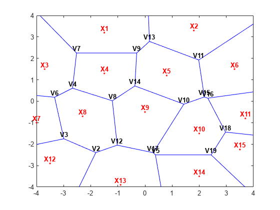
Highlight the points in red and assign the labels to the points.

hold on
plot(X(:,1),X(:,2),".r");
plabels = arrayfun(@(n){sprintf("X%d",n)},(1:size(X,1))');
text(X(:,1),X(:,2)+0.2,plabels,Color="r");

Compute the topology of the Voronoi diagram.

dt = delaunayTriangulation(X);
[V,R] = voronoiDiagram(dt);

V is a matrix representing the coordinates of the Voronoi vertices, which are the vertices are the end points of the Voronoi edges. Assign labels to the Voronoi vertices V. By convention the first vertex is at infinity.

numv = size(V,1);
vlabels = arrayfun(@(n){sprintf("V%d", n)},(2:numv)');
text(V(2:end,1),V(2:end,2)+.2,vlabels,Color="b");
hold off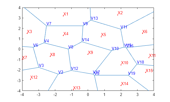

R is a vector cell array length size(X,1), representing the Voronoi region associated with each point. Hence, the Voronoi region associated with the point X(i) is R{i}. For example, R{9} gives the indices of the Voronoi vertices associated with the point site X9.

R{9}

ans = 1×5

     8    12    17    10    14

The indices of the Voronoi vertices are the indices with respect to the V array.

Similarly, R{4} gives the indices of the Voronoi vertices associated with the point site X4.

R{4}

ans = 1×5

     4     8    14     9     7

Alternatively, you can use the voronoin function to compute the topology of the Voronoi diagram.

[V,R]=voronoin(X);

This function supports computations for discrete points in N-D, where N ≥ 2, so you can use it for sets of points in 4-D and higher dimensions. For large data sets, this function might be slower than voronoiDiagram.

Note that the indices of the Voronoi vertices returned by voronoiDiagram and voronoin can differ.

R{9}

ans = 1×5

    17     5     2    10    15

R{4}

ans = 1×5

    19    17    15    16    18