Main Content

constantplane

Infinite plane in 3-D coordinates

Since R2024b

    Description

    constantplane(normal,offset) creates an infinite plane for highlighting slices or regions of 3-D plots. The plane satisfies the equation ax + by + cz = d, where the normal vector is [a b c] and the offset value is d. To create a plane that is perpendicular to the x-, y-, or z-axis, specify normal as "x", "y", or "z". To create a skewed plane, specify normal as a three-element vector.

    • To create one plane, specify one normal vector (either "x", "y", or "z", or a three-element vector) and a scalar offset value.

    • To create n planes, specify the normal vectors as the rows of an n-by-3 matrix or the columns of a 3-by-n matrix. Specify the offsets in an n-element vector.

    example

    constantplane(normal,offset,Name=Value) specifies properties of the plane using one or more name-value arguments. For example, constantplane([1 1 1],1,FaceColor="red") creates a red plane. If you create multiple planes, the property values apply to all of the planes. For a list of properties, see ConstantPlane Properties.

    example

    constantplane(ax,___) specifies the target axes for the plane. Specify ax as the first argument in any of the previous syntaxes.

    cp = constantplane(___) returns one or more ConstantPlane objects. Use cp to set properties of the planes after creating them. For a list of properties, see ConstantPlane Properties.

    example

    Examples

    collapse all

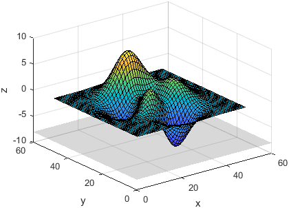
    Plot the peaks data set as a surface, and display the plane z=-8 below the surface.

    surf(peaks)
    constantplane("z",-8)
    xlabel("x")
    ylabel("y")
    zlabel("z")

    Surface plot with a plane underneath it

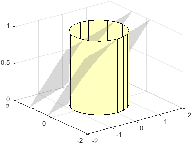
    Plot a cylinder with two planes that cut through the cylinder diagonally. Specify the plane normals as the rows of a 2-by-3 matrix. Specify the offsets as a two-element vector. Then adjust the x- and y-axes limits so you can see more of the planes.

    [X,Y,Z] = cylinder;
    surf(X,Y,Z,FaceColor=[1 1 0.75])
    normal = [-0.2 0.5 1; -0.2 0.5 1];
    offset = [0.5 1];
    constantplane(normal,offset)
    
    % Adjust x- and y-axes limits
    xlim([-2 2])
    ylim([-2 2])

    Cylinder intersecting with two diagonal planes

    You can modify aspects of a plane by setting properties. You can set properties by specifying name-value arguments when you call constantplane, or you can set properties later using dot notation.

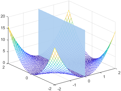
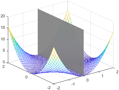
    For example, plot a surface and a vertical plane. Specify the opacity of the plane by setting the FaceAlpha name-value argument. Also, specify an output argument to store the ConstantPlane object.

    [X,Y] = meshgrid(-2:0.1:2);
    Z = X.^2 .* Y.^2;
    mesh(X,Y,Z)
    cp = constantplane("x",0,FaceAlpha=0.9);

    Mesh plot intersecting with a gray vertical plane

    Modify the appearance further by setting properties of the ConstantPlane object cp. Change the color to a shade of blue by setting the FaceColor property to a hexadecimal color code.

    cp.FaceColor = "#ABCDEF";

    Mesh plot intersecting with a light blue vertical plane

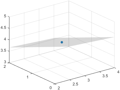
    The plane normal controls the orientation of the plane. Plot the point p = (3, 1, 4) by calling the scatter3 function. Create a normal vector, and define the offset as the dot product of the normal vector and the vector that points to p.

    p = [3 1 4];
    scatter3(p(1),p(2),p(3),"filled")
    normal = [1 2 3];
    offset = dot(normal,p); 
    constantplane(normal,offset)
    grid on

    Plane with a one blue marker in the center

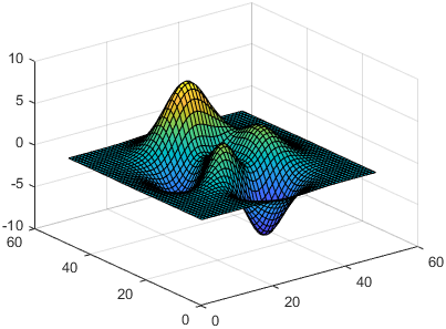
    Plot the peaks data set as a surface.

    surfdata = peaks;
    surf(surfdata)
    hold on

    Surface plot of the peaks data set

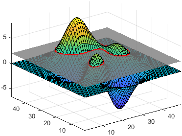
    Draw red contour lines that separate regions of the surface that are less than or equal to 2 from regions that are greater than or equal to 2. Set Zlocation to 2 to draw the contour lines at an altitude of z=2. Then draw a plane that cuts through the surface at z=2.

    levels = [2 2];
    contour(surfdata,[2 2],ZLocation=2,EdgeColor="red",LineWidth=2)
    constantplane("z",2,FaceAlpha=0.8)
    hold off

    Surface plot of peaks dataset with red contour lines and a translucent plane at z=2

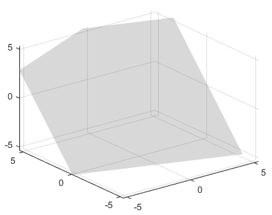
    Unlike many plotting functions, constantplane does not adjust the axes limits to include the plane. To display a plane without any additional data, calculate a set of axes limits that include part of the plane.

    For example, define a normal vector and an offset value for a plane. Then calculate the distance from the plane to the origin using dist = 2*offset/norm(normal).

    normal = [1 3 -2]; 
    offset = 5;
    dist = 2*offset/norm(normal);
    

    Display the plane, and set the x-, y-, and z-axes limits to [-2*dist 2*dist].

    constantplane(normal,offset)
    xlim([-2*dist 2*dist])
    ylim([-2*dist 2*dist])
    zlim([-2*dist 2*dist])
    grid on

    A plane by itself

    Input Arguments

    collapse all

    Normal vector, specified as one of these values:

    • "x", "y", or "z" — Abbreviations for the vectors [1 0 0], [0 1 0], and [0 0 1] respectively.

    • Three-element numeric vector — A normal vector for one plane.

    • n-by-3 or 3-by-n matrix — A matrix containing n normal vectors for displaying n planes. Specify the vectors as the rows of an n-by-3 matrix or the columns of a 3-by-n matrix. If you specify a 3-by-3 matrix, constantplane uses the columns of the matrix as the normal vectors.

    No plane appears if any components of the normal vector are NaN values or if the normal vector is the zero vector ([0 0 0]).

    Example: constantplane("x",0.5) creates a plane that is perpendicular to the x-axis and 0.5 unit from the origin.

    Example: constantplane([1 1 1],0.5) creates a plane using the normal vector [1 1 1] and an offset value of 0.5.

    Example: constantplane(["x" "y"],[0.5 0.5]) creates two perpendicular planes that intersect with the x- and y-axes, respectively, and each has an offset value of 0.5.

    Example: constantplane([1 0 0; 0 1 0],[0.5 0.5]) creates two perpendicular planes that intersect with the x- and y-axes, respectively. Each plane has an offset value of 0.5.

    Data Types: single | double | int8 | int16 | int32 | int64 | uint8 | uint16 | uint32 | uint64

    Offset value, which is the distance between the plane and the origin, specified as a numeric scalar or a vector. To create one plane, specify the offset value as a scalar. To create n planes, specify an n-element vector.

    No plane appears for an offset value of NaN.

    Example: constantplane("x",0.5) creates a plane that is perpendicular to the x-axis and 0.5 unit from the origin.

    Example: constantplane([2 2 0],1) creates a plane that is 1 unit away from the origin.

    Example: constantplane("y",[0.5 1]) creates two planes that intersect with the y-axis and are positioned 0.5 unit and 1 unit from the origin, respectively.

    Data Types: single | double | int8 | int16 | int32 | int64 | uint8 | uint16 | uint32 | uint64

    Target axes for the plane, specified as an Axes object. Use this argument if you want constantplane to plot into a specific Axes object instead of the current axes.

    Name-Value Arguments

    Specify optional pairs of arguments as Name1=Value1,...,NameN=ValueN, where Name is the argument name and Value is the corresponding value. Name-value arguments must appear after other arguments, but the order of the pairs does not matter.

    Example: constantplane([1 1 1],1,FaceColor="red") creates a red plane.

    Note

    The properties listed here are only a subset. For a complete list, see ConstantPlane Properties.

    Fill color, specified as an RGB triplet, a hexadecimal color code, or a color name.

    For a custom color, specify an RGB triplet or a hexadecimal color code.

    • An RGB triplet is a three-element row vector whose elements specify the intensities of the red, green, and blue components of the color. The intensities must be in the range [0,1], for example, [0.4 0.6 0.7].

    • A hexadecimal color code is a string scalar or character vector that starts with a hash symbol (#) followed by three or six hexadecimal digits, which can range from 0 to F. The values are not case sensitive. Therefore, the color codes "#FF8800", "#ff8800", "#F80", and "#f80" are equivalent.

    Alternatively, you can specify some common colors by name. This table lists the named color options, the equivalent RGB triplets, and hexadecimal color codes.

    Color NameShort NameRGB TripletHexadecimal Color CodeAppearance
    "red""r"[1 0 0]"#FF0000"

    Sample of the color red

    "green""g"[0 1 0]"#00FF00"

    Sample of the color green

    "blue""b"[0 0 1]"#0000FF"

    Sample of the color blue

    "cyan" "c"[0 1 1]"#00FFFF"

    Sample of the color cyan

    "magenta""m"[1 0 1]"#FF00FF"

    Sample of the color magenta

    "yellow""y"[1 1 0]"#FFFF00"

    Sample of the color yellow

    "black""k"[0 0 0]"#000000"

    Sample of the color black

    "white""w"[1 1 1]"#FFFFFF"

    Sample of the color white

    "none"Not applicableNot applicableNot applicableNo color

    Here are the RGB triplets and hexadecimal color codes for the default colors MATLAB® uses in many types of plots.

    RGB TripletHexadecimal Color CodeAppearance
    [0 0.4470 0.7410]"#0072BD"

    Sample of RGB triplet [0 0.4470 0.7410], which appears as dark blue

    [0.8500 0.3250 0.0980]"#D95319"

    Sample of RGB triplet [0.8500 0.3250 0.0980], which appears as dark orange

    [0.9290 0.6940 0.1250]"#EDB120"

    Sample of RGB triplet [0.9290 0.6940 0.1250], which appears as dark yellow

    [0.4940 0.1840 0.5560]"#7E2F8E"

    Sample of RGB triplet [0.4940 0.1840 0.5560], which appears as dark purple

    [0.4660 0.6740 0.1880]"#77AC30"

    Sample of RGB triplet [0.4660 0.6740 0.1880], which appears as medium green

    [0.3010 0.7450 0.9330]"#4DBEEE"

    Sample of RGB triplet [0.3010 0.7450 0.9330], which appears as light blue

    [0.6350 0.0780 0.1840]"#A2142F"

    Sample of RGB triplet [0.6350 0.0780 0.1840], which appears as dark red

    Fill color transparency, specified as a scalar in the range [0,1]. A value of 1 is opaque and 0 is completely transparent. Values between 0 and 1 are partially transparent.

    Version History

    Introduced in R2024b
    See Also

    Functions

    Properties