Visualize Models and Strategies

Use the Surface Viewer to

Visualize models and strategies
Display errors between the model and strategy
Display prediction error of the model
Create a movie to evaluate two variables at successive values of a third variable.
Print or export the display data

Access the Surface Viewer and Set Variable Ranges

To access the Surface Viewer, select Tools > Surface Viewer or click on the toolbar.

These are the main steps to view the model or feature using the Surface Viewer dialog box:

The model or feature selected when you open the Surface Viewer is displayed in the plot. If you have more than one model or feature, select what to display from the top Items list.
You can multiselect up to four items at once using Ctrl+click (the plot view on the right divides into a maximum of four plots). All the settings below the Items list apply to all plots. If one of the features selected in the Items list does not contain the appropriate input variables you select to plot, there is no plot for that item.
Select the ranges for the variables.
Choose the plot type to display. You can view surfaces, contour plots, single and multilines, movies, tables, and single values.
For example, as you view a feature, you can view either the strategy, the model associated with that feature, the error between the model and the strategy, or the prediction error if the model was imported from the Model Browser. You can also use one of these factors to shade the surface formed by one of the other factors, and you can select any two factors to display simultaneously as two surfaces.

The Surface Viewer does not work over continuous ranges, only at discrete points. Specify, for the model or feature, the discrete points you want to include in the display. You can display models or features over a range of points. To edit the displayed values of a variable, double-click in the value box for the appropriate variable.

Variables not being used for the axes plotted have a single value for that plot; to edit the displayed value for these variables you can type directly into the edit box after double-clicking.
For variables specified by the axes drop-down menus, the value box displays the range over which that variable is plotted and the number of points plotted across that range. To edit both the range and the number of points, double-click the value box. The Value Editor opens.

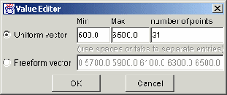
Here you can indicate the points to include in the display. You can specify

The minimum and maximum values and the number of points across that range by choosing Uniform Vector and typing in the edit boxes Min, Max, and Number of points.
Each discrete point at which you want to evaluate the model (or feature), by choosing Freeform vector, and then typing the required values.
For example, if you want to display the variable x at 0, 1, 7, 30, and 50, enter the following in the Freeform vector edit box, separated by tabs or spaces:
```
0 1 7 30 50
```

Click OK to apply your changes to the plot.

When you alter the variables, you can select whether you want the display to update automatically or not. You can toggle the automatic update on and off by selecting Tools > Auto-Evaluate. When you want to update the display, select Tools > Evaluate Now. Both of these options have equivalent toolbar buttons:

Display Point-by-Point Models in the Surface Viewer

When you are displaying a point-by-point model, you can select the operating point to display. When you are using point-by-point models, these are the points of interest you want to display.

To select the operating point to display in the Surface Viewer,

Select Tools > Select Operating Point (or the equivalent toolbar button). The Model Operating Points dialog box opens.
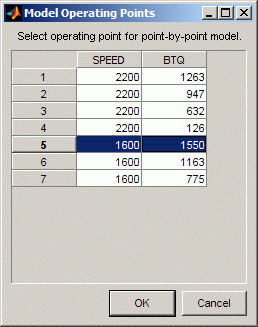
Select the operating point you want to display and click OK.

Surface Viewer snaps the display automatically to the selected point-by-point model operating point. When you select an operating point, Surface Viewer uses the model ranges for that operating point to set the local inputs (ranges and midpoints as applicable).

Introducing Error Displays

There are two different error displays available in the surface display options for primary and secondary surfaces and surface shading:

Error between the model and the strategy
Prediction error of the model

View Feature Error Data

When you are viewing a feature, this displays the error between the strategy and the model.

To display the error, select Error (strategy-model) from the drop-down menu for primary or secondary surface. You can also choose to shade your primary surface with the error by using the Surface 1 Shading menu.

To view the error statistics, select View > Statistics. This opens a dialog box with a list of the summary statistics for the error between model or feature.

View Prediction Error Data

If the model is imported from the Model Browser, it is possible to display the prediction error (PE) data.

Prediction Error Variance (PEV) is a useful way to investigate the predictive capability of your model. It gives a measure of the precision of a model prediction. You can examine the PEV in the Model Browser, both in the Prediction Error Variance Viewer and to shade surfaces in the Model Selection and Model Evaluation views. Here you can examine the PEV of designs and models. When you export the model to CAGE, you can see this data in the Surface Viewer in the Prediction Error option. See the Model Browser GUI Reference and Technical Documents for details about the calculation of Prediction Error.

Viewing the Prediction Error. Select Prediction Error from the drop-down display menus for primary or secondary surfaces. You can also choose Prediction Error to shade your primary surface. As with all other plots, you can view the statistics for the Prediction Error displayed by selecting View > Statistics. The mean, standard deviation, and so on, are calculated over the range specified in the variable value boxes.

Create a Movie Using the Surface Viewer

You can make a movie. This enables you to view the model or feature as it steps through several values of a variable. For example, if you want to view a feature calibrated for maximum brake torque (MBT) as it varies over exhaust gas recycling (EGR), you can make a movie of the feature.
Choose Movie from the Plot Type drop-down menu in the Data to Plot pane.
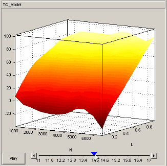
The movie option allows you to see an evaluation over two variables at successive values of a third variable. For example, a model of torque might have speed (N), load (L), and air/fuel ratio (A) as inputs.
The movie option allows you to view how the torque model behaves over the ranges of speed and load for successive values of air/fuel ratio.
1. Select three variables from the X-axis, Y-axis, and Time drop-down menus, to indicate which variable you want to display. You can view the model surface plotted across the range of two variables, and define the third variable as "time" to see the model surface change across the third variable range.
2. Define the variable ranges using the Value boxes for the inputs.
3. Select the check box to mark boundaries if available.
4. Click Play.
5. You can click the buttons at each end of the progress bar under the plot to step through the movie, or click anywhere along the bar (or click and drag the blue pointer) to display a particular point in the movie. You can rotate the plot (including during play).

Print and Export the Display

To print the display, select File -> Print, or you can select Print to Figure. Selecting File > Copy to Clipboard copies the plot image to the clipboard. This is useful if you want to place plot images into other applications. These print options also have equivalent toolbar buttons.

You can also export the display data to a comma-separated variable file.

To export the display, select File > Export to CSV. The currently selected option is exported. The primary input to the first plot is exported (this is the top left if you have multiple plots). The output is the values at the grid of points specified by the current ranges and input values. The inputs for shading and secondary surfaces are not exported.

You cannot print table plots, but you can click and drag to select cells and press Ctrl-C to copy the values to the clipboard, or you can export them to CSV files and then load them into Excel.