Explore Local Model Types
Alternative Local Model Types
First, try fitting the defaults using the Fit models common task button.
If you want to try alternative local model types, select the response node, then in the Common Tasks pane, click New Local Model. This opens the Local Model Setup dialog box. Browse the model types on this page.
To examine fits, see Assess Local Models.
The available models depend on the number of input factors. Polynomial, polynomial spline, truncated power series, free knot spline, and growth models are for one factor only.
You can choose additional response features at this stage using the Response Features tab of the Local Model Setup dialog box. These can also be added later. The Model Browser chooses sufficient response features for the current model.
See each local model type for statistical details and available response features.
See also
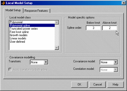
Local Model Class: Polynomials and Polynomial Splines
Polynomials
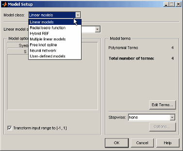
At the local level, if you have one input factor, you can choose Polynomial directly from the list of local model classes. Here you can choose the order of polynomials used, and you can define a datum model for this kind of local model.
If there is more than one input factor, you can choose Linear Models from the Local Model Class list, then you can choose Polynomial or Hybrid Spline. This is a different polynomial model where you can change more settings such as Stepwise, the Term Editor (where you can remove any model terms) and you can choose different orders for different factors (as with the global level polynomial models). See Local Model Class: Linear Models.
Different response features are available for this polynomial model and the Linear Models: Polynomial choice. You can view these by clicking the Response Features tab on the Local Model Setup dialog box. Single input polynomials can have a datum model, and you can define response features relative to the datum. See Datum Models.
The following response features are permitted for the polynomial model class:
Location of the maximum or minimum value.
Value of the fit function at a user-specified x-ordinate. When datum models are used, the value is relative to the datum (for example, mbt - x).
The nth derivative at a user-specified x-ordinate, for n = 1, 2, ..., d where d is the degree of the polynomial.
See the global model section Polynomials for a general description of polynomial models.
Polynomial Spline
A spline is a piecewise polynomial, where different sections of polynomial are fitted smoothly together. The location of each break is called a knot. Polynomial splines are essential for modeling torque/spark curves.
This model has only one knot. You can choose the orders of the polynomials above and below the knot. See also Hybrid Splines. These global models also use splines, but use the same order polynomial throughout.
Polynomial splines are only available for single input factors. The following example shows a typical torque/spark curve, which requires a spline to fit properly. The knot is shown as a red spot at the maximum, and the curvature above and below the knot is different. In this case, there is a cubic basis function below the knot and a quadratic above.
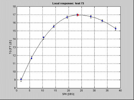
To model responses that are characterized in appearance by a single and well-defined stationary point with asymmetrical curvature either side of the local minimum or maximum, define the following spline class,
![]()
where k is the knot location, ![]() denotes a regression coefficient,
denotes a regression coefficient, ![]() ,
, ![]() .
.
where c is the user-specified degree for the left polynomial, h is the user-specified degree for the right polynomial, and the subscripts Low and High denote to the left (below) and right of (above) the knot, respectively.
Excluding terms in ![]() and
and ![]() ensures that the first derivative at the knot position is
continuous. In addition, by definition the constant
ensures that the first derivative at the knot position is
continuous. In addition, by definition the constant ![]() must be equal to the value of the fit function at the knot, that
is, the value at the stationary point.
must be equal to the value of the fit function at the knot, that
is, the value at the stationary point.
For this model class, response features can be chosen as
Fit constants

Knot position

Value of the fit function at a user-specified delta

from the knot position
 if the datum is defined, otherwise the value is
absolute.
if the datum is defined, otherwise the value is
absolute.Difference between the value of the fit function at a user-specified delta from the knot position and the value of the fit function at the knot
Local Model Class: Linear Models
Select Linear Models and then click
Setup.
You can now set up polynomial or hybrid spline models. The settings are exactly the same as the global linear models.
These models are for multiple input factors - for single input factors you can use a different polynomial model from the Local Model Class list, where you can only change the polynomial order. See Local Model Class: Polynomials and Polynomial Splines.
If there is more than one input factor, you can choose Linear Models from the Local Model Class list, then you can choose Polynomial or Hybrid Spline. This polynomial is a different model where you can change more settings such as Stepwise, the Term Editor (where you can remove any model terms) and you can choose different orders for different factors (as with the global level polynomial models).
See Global Linear Models: Polynomials and Hybrid Splines for details.
By default inputs are transformed to [-1, 1] before fitting and evaluating polynomials. This is important as differences in scales between inputs can cause numerical problems. Generally it is a good idea to transform inputs as this alleviates problems with variables of different scales. In some circumstances, you might be concerned with the values of polynomials (for example if your strategy requires raw polynomial coefficients). In this case, you can clear the Transform input range check box to use untransformed units to calculate natural polynomials.
Different response features are available for this Linear Models: Polynomial model and the other Polynomial choice (for single input factors). You can view these by clicking the Response Features tab on the Local Model Setup dialog box. Single input polynomials can have a datum model, and you can define response features relative to the datum. See Datum Models.
These linear models are labeled Quadratic,
Cubic, and so on, on the test plan block diagram. The single input
type of polynomials are labeled Poly2, Poly3, and
so on. For higher orders, both types are labeled Poly
n.
Local Model Class: Truncated Power Series
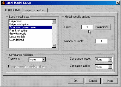
This is only available for a single input factor.
You can choose the order of the polynomial basis function and the number of knots for Truncated Power Series Basis Splines. A spline is a piecewise polynomial, where different sections of polynomial are fitted smoothly together. The point of each break is called a knot. The truncated power series changes the coefficient for the highest power when the input passes above the knot value.
It is truncated because the power series is an approximation to an infinite sum of polynomial terms. You can use infinite sums to approximate arbitrary functions, but clearly it is not feasible to fit all the coefficients.
Click Polynomial to see (and remove, if you want) the polynomial terms. One use of the remove polynomial term function is to make the function linear until the knot, and then quadratic above the knot. In this case, remove the quadratic coefficient.
See also
Polynomial Spline, where you can choose different order basis functions either side of the knot
Hybrid Splines, a global model where you can choose a spline order for one of the factors (the rest have polynomials fitted)
Local Model Class: Free Knot Spline, free knot splines, where you can choose the number of knots and the order of the basis functions
Truncated Power Series Basis (TPSBS) Splines
A general class of spline functions with arbitrary (but strictly increasing) knot sequence:
![]() :
: ![]()
This defines a spline of order m with knot sequence ![]()
For this model class, response features can be chosen as
Fit constants
Knot position vector
 .
.Value of the fit function
 at a user-specified value
Value of the nth derivative of the fit function with respect to xj
 at a user-specified value
  , with n = 1, 2, ..., m-2
You can remove any of the polynomial terms from the model.
Local Model Class: Free Knot Spline
These are the same as the Global Model Class: Free Knot Spline (which is also only available for one input factor). See the global free knot splines for an example curve shape.
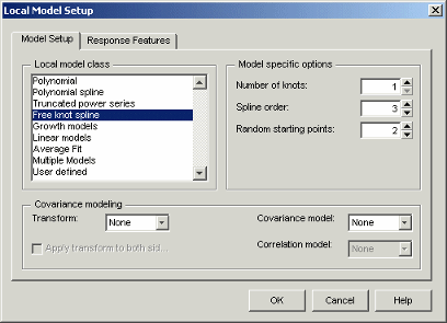
A spline is a piecewise polynomial, where different sections of polynomial are fitted smoothly together. The point of the join is called the knot.
You can choose the number of knots. You can choose the order of polynomial fitted (in all curve sections) from 1 to 3. The default is cubic.
You can set the number of Random starting points. These are the number of initial guesses at the knot positions.
See also
Polynomial Spline, where you can choose different order basis functions for either side of the knot
Local Model Class: Truncated Power Series, where you can choose the order of the basis function
Hybrid Splines, a global model where you can choose a spline order for one of the factors (the rest have polynomials fitted)
Free Knot Splines
The ![]() basis is not the best suited for the purposes of estimation and
evaluation, as the design matrix might be poorly conditioned. In addition, the number
of arithmetic operations required to evaluate the spline function depends on the
location of
basis is not the best suited for the purposes of estimation and
evaluation, as the design matrix might be poorly conditioned. In addition, the number
of arithmetic operations required to evaluate the spline function depends on the
location of ![]() relative to the knots. These properties can lead to numeric
inaccuracies, especially when the number of knots is large. You can reduce such
problems by employing B-splines.
relative to the knots. These properties can lead to numeric
inaccuracies, especially when the number of knots is large. You can reduce such
problems by employing B-splines.
The most important aspect is that for moderate m the design matrix expressed in terms of B-splines is relatively well conditioned.
For this model class, response features can be chosen as
Fit constants
Knot position vector
 .
.
Value of the fit function ![]() at a user specified value
at a user specified value ![]()
Local Model Class: Growth Models
Growth models have several varieties available. They are only available for single input factors.
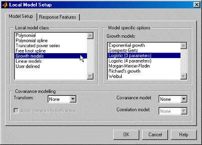
These are all varieties of sigmoidal curves between two asymptotes, like the following example.
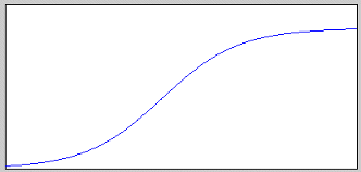
Growth models are often the most appropriate curve shape for air charge engine modeling.
See the following sections for mathematical details on the differences between these growth models:
Three Parameter Logistic Model
The equation defines the three parameter logistic curve.
where ![]() is the final size achieved, is a scale parameter, and
is the final size achieved, is a scale parameter, and ![]() is the x-ordinate of the point of inflection of the curve.
is the x-ordinate of the point of inflection of the curve.
The curve has asymptotes yj = 0 as
xj
-∞ and ![]() as xj ∞. Growth rate is at a maximum when
yj = α/2, which occurs when xj = . Maximum growth rate corresponds to
as xj ∞. Growth rate is at a maximum when
yj = α/2, which occurs when xj = . Maximum growth rate corresponds to
![]()
The following constraints apply to the fit coefficients:
α > 0, , .
The response feature vector g for the three parameter logistic
function is defined as
Morgan-Mercer-Flodin Model
This equation defines the Morgan-Mercer-Flodin (MMF) growth model.
where α is the value of the upper asymptote, β is the value of the lower asymptote, is a scaling parameter, and δ is a parameter that controls the location of the point of inflection for the curve. The point of inflection is located at
![]()
![]()
for ![]()
There is no point of inflection for δ < 1. All the MMF curves are sublogistic, in the sense that the point of inflection is always located below 50% growth (0.5α). The following constraints apply to the fit coefficient values:
α > 0, β > 0, > 0, δ > 0
α > β
This equation provides the response feature vector g.
Four-Parameter Logistic Curve
This equation defines the four-parameter logistic model.
with constraints ![]() ,
, ![]() and
and ![]() . Again,
. Again, ![]() is the value of the upper asymptote,
is the value of the upper asymptote, ![]() is a scaling factor, and
is a scaling factor, and ![]() is a factor that locates the x-ordinate of the point of
inflection at
is a factor that locates the x-ordinate of the point of
inflection at
The following constraints apply to the fit coefficient values:
All parameters > 0
α > β
This is the available response feature vector:
Richards Curves
This equation defines the Richards curves family of growth models.
![]() δ ≠ 1
δ ≠ 1
where α is the upper asymptote, is the location of the point of inflection on the x axis, is a scaling factor, and δ is a parameter that indirectly locates the point of inflection.
The y-ordinate of the point of inflection is determined from
![]()
![]()
Richards also derived the average normalized growth rate for the curve as
![]()
The following constraints apply to the fit coefficient values:
α > 0, > 0, > 0, δ > 0
α >
δ ≠ 1
Finally, the response feature vector g for Richards family of
growth curves is defined as
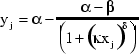
Weibul Growth Curve
This equation defines the Weibul growth curve.
![]()
where ![]() is the value of the upper curve asymptote,
is the value of the upper curve asymptote, ![]() is the value of the lower curve asymptote,
is the value of the lower curve asymptote, ![]() is a scaling parameter, and
is a scaling parameter, and ![]() is a parameter that controls the x-ordinate for the point of
inflection for the curve at
is a parameter that controls the x-ordinate for the point of
inflection for the curve at
![]()
The following constraints apply to the curve fit parameters:
α > 0, β > 0, > 0, δ > 0
α > β
The associated response feature vector is
Exponential Growth Curve
This equation defines the exponential growth model.
![]()
where α is the value of the upper asymptote, β is the initial size, and is a scale parameter (time constant controlling the growth rate). The following constraints apply to the fit coefficients:
α > 0, β > 0, > 0
α > β
The response feature vector g for the exponential growth model
is defined as
![]()
Gompertz Growth Model
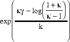
Another useful formulation that does not exhibit a symmetric point of inflection is the Gompertz growth model. The defining equation is
![]()
where α is the final size, is a scaling factor, and is the x-ordinate of the point of inflection. The corresponding y-ordinate of the point of inflection occurs at
![]()
With maximum growth rate
![]()
The following constraints apply to the selection of parameter values for the Gompertz model:
α > 0, > 0, > 0.
The response feature vector g for the Gompertz growth model is
defined as
Local Model Class: User-Defined Models
You can create user-defined models to use for local, global, or one-stage models.
The user-defined model type allows you to define your equation in a file to use for fitting in the toolbox.
To create and check in a user-defined model:
Copy the user-defined template file (
functemplate.m) to a location on the MATLAB® path (but not undermatlabroot\toolbox\mbc<matlabroot>\toolbox\mbc\mbcmodels\@xregusermod\functemplate.m
Modify the copy of the template file for your model. Code all the compulsory functions. The template comments describe all the compulsory and optional functions.
It is not compulsory to modify every optional section. If you do not want to use an optional section, leave it unmodified.
Check your model into the toolbox with this command:
m = checkin(xregusermod,'MfileName',TestInputData)
Note
Your user-defined models can have as many factors as you choose.
After you check in your user-defined models, they appear as options on the Model Setup dialog box when you are using data with the right number of factors.
To remove your checked-in model from the toolbox, enter:
remove(xregusermod,'MfileName')
Note
If any of your global models are user-defined you cannot use MLE (maximum likelihood estimation) for your two-stage model.
You can examine this example user-defined model file as a guide:
<MATLAB root>\toolbox\mbc\mbcmodels\@xregusermod\weibul.m
This file defines the local model Weibul (Growth Model) in the toolbox and hence should not be changed. Make sure that you do not overwrite the file. If you alter the file, save it under another name.
Examine the Example User-Defined Model
This example demonstrates how to create a user-defined model for the Weibul function:
y = alpha - (alpha - beta).*exp(-(kappa.*x).^delta)
Open the following example file
<MATLAB root>\toolbox\mbc\mbcmodels\@xregusermod\weibul.m
Observe that the file is called by the toolbox using
varargout= weibul(m,x,varargin)
Where the variables are given by
m = the xregusermod object
x = input data as a column vector for fast eval
The first function in the template file is a vectorized evaluation of the function. First, the model parameters are extracted:
b= double(m);
Then, the evaluation occurs:
y = b(1) - (b(1)-b(2)).*exp(-(b(3).*x).^b(4));
Note
The parameters are always referred to and declared in the same order.
Compulsory Local Functions. Edit these local functions as follows:
Enter the number of input factors. For functions y = f(x) this is 1.
function n= i_nfactors(U,b)
n= 1;
Enter the number of fitted parameters. In this example, there are four parameters in the Weibul model.
function n= i_numparams(U,b)
n= 4;
The following local function returns a column vector of initial values
(param) for the parameters to fit. The initial values can be
defined to be data-dependent; hence there is a flag to signal if the data is not
worth fitting (OK). In weibul.m there is a
routine for calculating a data-dependent initial parameter estimate. If no data is
supplied, the default parameter values are used.
function [param,OK]= i_initial(U,b,X,Y)
param= [2 1 2 5]';
OK=1;
Optional Local Functions. You can use the following optional local functions to set additional parameters
You can state lower and upper bounds for the model parameters. These bounds appear in the same order that the parameters are declared and used throughout the template file.
function [LB,UB,A,c,nlcon,optparams]=i_constraints(U,b,varargin)
LB=[eps eps eps eps]';
UB=[1e10 1e10 1e10 1e10]';
You can also define linear constraints on the parameters. This code produces the constraint (–alpha+beta) is less than or equal to zero:
A= [-1 1 0 0];
c= [0];
nlcondefines the number of nonlinear constraints (here declared to be zero). If the number of nonlinear constraints is not zero, the nonlinear constraints are calculated ini_nlconstraints.nlcon= 0;
optparamsdefines any optional parameters. No optional parameters are declared for the cost function.optparams= [];
i_foptionsdefines the fit options. The fit options are always based on the inputfopts. See MATLAB help on theoptimsetoroptimoptionsfunctions for more information on fit options. When there are no constraints, the toolbox uses the MATLAB functionlsqnonlinfor fitting, otherwisefminconis used.function fopts= i_foptions(U,b,fopts) fopts= optimset(fopts,'Display','none');
i_jacobiancan supply an analytic Jacobian to speed up the fitting algorithm.function J= i_jacobian(U,b,x) x = x(:); J= zeros(length(x),4); a=b(1); beta=b(2); k=b(3); d=b(4); ekd= exp(-(k.*x).^d); j2= (a-beta).*(k.*x).^d.*ekd; J(:,1)= 1-ekd; J(:,2)= ekd; J(:,3)= j2.*d./k; J(:,4)= j2.*log(k.*x);
i_labelsdefines the labels used on plots. You can use LaTeX notation and it is formatted.function c= i_labels(U,b) c={'\alpha','\beta','\kappa','\delta'};i_charis the display equation string and can contain LaTeX expressions. The current values of model parameters appear.function str= i_char(U,b) s= get(U,'symbol'); str=sprintf('%.3g - (%.3g-%.3g)*exp(-(%.3g*x)^{%.3g})',... b([1 1 2 3]), detex(s{1}), b(4));i_str_funcdisplays the function definition with labels appearing in place of the parameters (not numerical values).function str= i_str_func(U,b, TeX) s= get(U,'symbol'); if nargin == 2 || TeX s = detex(s) end % This can contain TeX expressions supported by HG text objects lab= labels(U); str= sprintf('%s - (%s - %s)*exp(-(%s*%s)^{%s})',... lab{1},lab{1},lab{2},lab{3},s{1},lab{4});i_rfnamesdefines response feature names. This example shows a defined response feature that is not one of the parameters (in this case it is also nonlinear).You do not need to define
rname(it can return an empty cell array).function [rname, default] = i_rfnames(U,b) % response feature names rname= {'inflex'}; if nargout>1 default = [1 2 5 4]; %{'Alpha','Beta','Inflex','Delta'}; endi_rfvalsdefines response feature values. This example defines the response feature labeled asINFLEXin previous step. The Jacobian matrix is also defined here asdG.function [rf,dG]= i_rfvals(U,b) %I_RECONSTRUCT nonlinear reconstruction % % p = i_reconstruct(m,b,Yrf,dG,rfuser) % Inputs % Yrf response feature values % dG Jacobian of response features with respect to % parameters % rfuser index to the user-defined response features % so you can find out which response features % are which. rfuser(i) = 0 if the rf is a parameter. % % If all response features are linear in model parameters % then you do not need to define 'i_reconstruct'. % this is an example of how to implement a nonlinear response % feature definition K = b(3); D = b(4); if D>=1 rf= (1/K)*((D-1)/D)^(1/D); else rf= NaN; end if nargout>1 % Jacobian of response features with respect to model % parameters if D>=1 dG= [0, 0, -((D-1)/D)^(1/D)/K^2,... 1/K*((D-1)/D)^(1/D)*(-1/D^2*log((D-1)/D)+... (1/D-(D-1)/D^2)/(D-1))]; else dG= [0, 0, 1 1]; end endThe
i_reconstructlocal function allows the model parameters to be reconstructed from the response features that have been given. If all response features are linear in the parameters, then you do not need to define this function. The code first identifies which response features (if any) are user defined.
function p= i_reconstruct(U,b,Yrf,dG,rfuser)
%I_RECONSTRUCT nonlinear reconstruction
%
% p = i_reconstruct(m,b,Yrf,dG,rfuser)
%  Inputs
%     Yrf   response feature values
%     dG    default Jacobian of response features
%     rfuser index to the user-defined response features so you can find
%     out which response features are which. rfuser(i) = 0 if the
%     rf is a parameter.
%
% If all response features are linear in model parameters then you do not
% need to define 'i_reconstruct'.

% reconstruct linear response features using this line
p= Yrf/dG';

% find which response feature is a nonlinear user-defined response feature
f= rfuser>size(p,2);
if ~any(rfuser==3)
   % need to use delta (must be > 1) for reconstruction to work
   p(:,4)= max(p(:,4),1+16*eps);

   p(:,3)= ((p(:,4)-1)./p(:,4)).^(1./p(:,4))./Yrf(:,f);
end
Check the Model into the Toolbox
After you create a user-defined model file, save it somewhere on the path.
Check in the model. The check in process ensures that the model you have defined provides an interface that allows the toolbox to evaluate and fit it. If the checkin procedure succeeds, the toolbox registers the model and makes it available for fitting when you use appropriate input data.
At the command-line, with the example file on the path, you need to create a model
and some input data, then call checkin. For the user-defined
Weibul function, call checkin with the example model, its name,
and some appropriate data.
checkin(xregusermod, 'weibul', [0.1:0.01:0.2]');
This returns some command-line output, and a figure appears with the model name and variable names displayed over graphs of input and model evaluation output. The final command-line output:
Model successfully registered for
Model-Based Calibration Toolbox software.
Verify That the Model Is Checked In
To verify a user-defined model is checked in to the toolbox:
Start the Model Browser and load data that has the necessary format to evaluate your user-defined model.
Set up a Test Plan with
NStage1 input factors, whereNis the number of input factors defined ini_nfactors.Open the Local Model Setup dialog box, and select User-defined models in the Local Model Class list. Your user-defined model should appear in the right list.
To verify that the weibul example user-defined model is
checked in:
Open
gasoline_project.mat, and select thePS22test plan node in the tree.Double-click the Local Model icon in the test plan diagram.
In the Local Model Setup dialog box, select User-defined models in the Local Model Class list. The
Weibuluser-defined model appears in the right list, as checked in.
Recover from Editing Errors
If you modify the file that defines a checked-in model that you are currently using, the Model Browser tries to continue.
If the user-defined model has serious errors (e.g., you have altered the number of inputs or parameters, model evaluation, or the file cannot be found), the Model Browser changes the status of the current model to 'Not fitted'.
To recover from this state, first correct the problem in the file. Then (for Local Models) you can select Model > Fit Local to refit. You do not need to check the model in again, but if you have problems the error messages produced during a checkin might be useful in diagnosing faults.
If there is a minor fault with the file, then the Model Browser continues, using
default values. Minor errors can include items such as label definitions, that is,
faults in i_char, i_label,
i_str_func, or i_foptions. A message appears
in the command window providing details of these faults.
Local Model Class: Transient Models
Use transient models for local, global, or one-stage models. The toolbox supports
transient models with multiple input factors where time is one of the factors. You can
define a dynamic model using Simulink® software and a file that describes parameters to fit in this model. The
toolbox provides an example called fuelPuddle which is already
checked in to the toolbox. You can use this example for modeling. The example provided
requires two input factors. The process of creating and checking in your own transient
models is described in the following sections using this example.
Locate the example Simulink model:
<MATLAB root>\toolbox\mbc\mbcsimulink\fuelPuddle
and the example user-defined transient model file:
<MATLAB root>\toolbox\mbc\mbcmodels\@xregtransient\fuelPuddle.m
Create Folders
You can define a dynamic model using a Simulink model and a user-defined transient model file that describes parameters to fit in this model. Create folders for these files that are on the MATLAB path. Then, you must check the files into the Model-Based Calibration Toolbox™ product before you can use them for modeling.
Create a folder and add it to the MATLAB path.
For example:
D:\MyTransient.Put your Simulink model in this folder. See Create Simulink Model.
Inside the new folder, create a folder called @xregtransient. (e.g., D:\MyTransient\@xregtransient). You must call this folder @xregtransient.
Put your user-defined transient model file in the new @xregtransient folder. This file must have the same name as your Simulink model. See Create a User-Defined Transient Model File.
Create Simulink Model
Create a Simulink model to represent your transient system.
Simulink inports represent the model inputs. Time is the first input to the model in Model-Based Calibration Toolbox software, but it is not an inport in the model. The model output is represented by a Simulink output. Only one scalar output is supported in the Model Browser.
Your Simulink model must have some free parameters that Model-Based Calibration Toolbox software will fit by nonlinear least squares. Use the same variable names in the model and the user-defined transient model file.
The Simulink model for the fuelPuddle example appears in the
following figure. You will examine the example file (fuelPuddle.m)
in a later section.
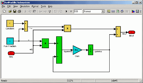
The block labels are not important. The model returns a single scalar output (here
labeled “Mcyl”).
The toolbox defines the model parameters in the Model Workspace. You can see this
in the Model Explorer. A vector of all parameters called p is also
available.
Model Requirements. For both continuous and discrete models, the following rules apply:
For Simulink models with a Fixed Step solver the step size is set to the sample time of the data.
For Variable step solvers the simulation step size is set by the Simulink model.
You see an error if the size of the output from simulating the Simulink model does not does not match the size of the input data provided by the toolbox.
Create a User-Defined Transient Model File
Define a transient model file for your Simulink model, and this file must have the same name as your Simulink model.
Copy the transient model template file, found at:
Copy the file to the new<MATLAB root>\toolbox\mbc\mbcmodels\@xregtransient\functemplate.m
MyTransientfolder\@xregtransientModify the copy of the template file for your model.
The commented code describes the compulsory and optional functions available in the template file.
You do not have to modify every section. If you do not want to use an optional section, leave it unmodified, and the defaults are sufficient.
Open the example file fuelPuddle.m (for the
fuelPuddle model) to examine the code described in the
following sections. Find the file here:
<MATLAB root>\toolbox\mbc\mbcmodels\@xregtransient\fuelPuddle.m
Compulsory Local Functions
Specify the following local functions:
Specify the parameters of the Simulink model to fit.
function vars= i_simvars(m,b,varargin);
vars = {'tau','x'};
This local function must return a cell array of strings. These are the parameter names that the Simulink model requires from the workspace. These strings must match the parameter names declared in the Simulink model.
If your Simulink model requires constant parameters to be defined, do so here:
function [vars,vals]= i_simconstants(m,b,varargin);
vars = {};
vals = [];
These are constant parameters required by the Simulink model from the workspace, and are not fitted. These parameters must be the same as those in the Simulink model, and all names must match. Here
fuelPuddlerequires no such parameters, and returns an empty cell array and empty matrix.Specify Initial conditions for the integrators.
function [ic]= i_initcond(m,b,X);
ic=[];
Initial conditions are based on the current parameters, and inputs could be calculated here. Leaving ic = [] means that Simulink uses the definition of initial conditions in the Simulink model.
Specify the number of input factors, including time.
function n= i_nfactors(m,b);
n= 2;
Time is the first input for transient models.
fuelPuddlehas the inputX = [t, u(t)], and so the number of input factors is 2.This local function returns a column vector of initial values for the fitted parameters.
function [b0,OK]= i_initial(m,b,X,Y)
b0= [0.5 0.1]';
OK=1;
Check
narginbefore using X and Y as this local function is called with 2 or 4 parameters: (m,b) or (m,b,X,Y).You could do some calculations here to estimate good initial values from the X, Y data. The initial values can be defined to be data dependent, hence there is an OK flag to signal if the data is not worth fitting. The example defines some default initial values for
xandtau.
Optional Local Functions
You do not need to edit the remaining local functions unless they are required. The comments in the code describe the role of each function. You use these functions most often when you are creating a user-defined model (see Local Model Class: User-Defined Models).
These labels are used on plots:
function c= i_labels(m,b)
b= {'\tau','x'};
You can use LaTeX notation, and it is correctly formatted. By default, the
variable names defined in i_simvars are used to specify parameter
names.
Check In to Toolbox
Having created a Simulink model and the corresponding function file, you must save each on the path, as described in Create Folders.
To ensure that the transient model you have defined provides an interface that allows the toolbox to evaluate and fit it, you check in the model. If this procedure succeeds, the toolbox registers the model and makes it available for fitting when you use appropriate input data.
At the command-line, with both template file and Simulink models on the path, create some input data, then call
checkin. The procedure follows.
Create some appropriate input data. The particular data used is not important; you are using it only to check whether the model can be evaluated.
For the
fuelPuddleexample, enter the following input at the command-line:TestInputData = [0:0.1:10; ones(1,101)]';
Call
checkinwith the transient model, its name, and the data. For the example, enter:m = checkin(xregtransient,'fuelPuddle',TestInputData)
The string you use for your new transient model name appears in the Model Setup dialog box when you set up transient models using the appropriate number of inputs.
xregtransientcreates a transient model object suitable for use in checking in and removing from the toolbox.
A successful checkin creates some command-line output, and a figure appears with
the model name and variable names displayed over graphs of input and model evaluation
output. The final command-line output (if checkin is called with a
semicolon as in the previous example) is
Model successfully registered for
Model-Based Calibration Toolbox software
Note
You might see errors if you modify the file or model that defines a checked-in transient model that you are currently using in the Model Browser. See Recover from Editing Errors.
Using and Removing Transient Models
The fuelPuddle model is already checked in for you to use. Open
the Model Browser and load data that has the necessary format to evaluate this
transient model (two local inputs). Time input data must be increasing.
Create a Test Plan with two local input factors (the same number of input factors
required by the fuelPuddle model). The Local Model Setup dialog
box now offers the following options:
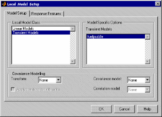
Select the fuelpuddle model, and click
OK.
On building a response model with fuelPuddle as the local
model, the toolbox fits the two parameters tau and
x across all the tests.
Removing Checked-In Models. To remove a checked-in model, close the Model Browser, and type the following command at the command-line:
remove(xregtransient, 'ModelName')
When you restart the toolbox, the command removes the checked-in transient model.
Local Model Class: Average Fit
You can use this local model class to fit the same model to all tests. Sometimes it is desirable to try to fit a single one-stage model to two-stage data (for example, fitting an RBF over the whole operating region of spark, speed, load, air/fuel ratio and exhaust gas recirculation). However, it can still be useful to be able to examine the model fit on a test-by-test basis. You can use Average Fit for this purpose.
Select Average Fit and click Setup.
The Model Setup dialog box appears.
In the Model class drop-down menu is a list of available models. This list contains the same models that you would find in the global model setup of a one-stage model. Note the number of inputs changes which models are available. A local model with only one input can access all the models.
The Average Fit local model class allows you to use any of these global model options to fit to all tests. In the same way that global models are fitted to all the data simultaneously, using average fit allows you to fit the same model to every test in your data, instead of fitting a separate local model for each test.
The advantage of this is that you can use these one stage models to fit your data while also being able to view the fit to each test individually. Set up your global model with an input such as record number or a dummy variable. Make all the variables you want to model local inputs. It does not matter what dummy variable or model type you use for the global input - it is only there to distinguish the Local Average Fit model from a one-stage model. The dummy global variable has no influence on the model fit. The Average Fit model is fitted in the same way as a one-stage model (across all tests simultaneously) but the main difference is that you can analyze the fit to each test individually. You cannot perform such analysis when fitting one-stage models.
Note
No two-stage model is available with local Average Fit models, and you cannot use covariance modeling.
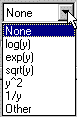
Transforms
The following example shows the transforms available.
Input transformation can be useful for modeling. For example, if you are trying to fit
![]()
using the log transform turns this into a linear
regression:
![]()
Transforms available are logarithmic, exponential, square root, ![]() ,
, ![]() , and
, and Other. If you choose
Other, an edit box appears and you can enter a function.
Apply transform to both sides is only available for nonlinear models, and transforms both the input and the output. This is good for changing the error structure without changing the model function. For instance, a log transform might make the errors relatively smaller for higher values of x. Where there is heteroscedasticity, as in the Covariance Modeling example, this transform can sometimes remove the problem.
Covariance Modeling
This frame is visible no matter what form of local model is selected in the list.
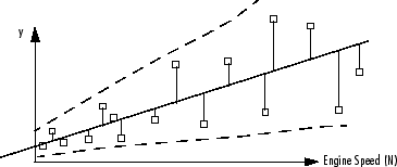
Covariance modeling is used when there is heteroscedasticity. This means that the variance around the regression line is not the same for all values of the predictor variable, for example, where lower values of engine speed have a smaller error, and higher values have larger errors. If so, data points at low speed are statistically more trustworthy, and should be given greater weight when modeling. Covariance models are used to capture this structure in the errors.
You can fit a model by finding the smallest least squares error statistic when there
is homoscedasticity (the variance has no relationship to the variables). Least squares
fitting tries to minimize the least squares error statistic![]() , where
, where ![]() .
.
is the error squared at point i.
When there is heteroscedasticity, covariance modeling weights the errors in favor of the more statistically useful points (in this example, at low engine speed N). The weights are determined using a function of the form
![]()
where ![]() is a function of the predictive variable (in this example, engine
speed N).
is a function of the predictive variable (in this example, engine
speed N).
There are three covariance model types.
Power
These determine the weights using a function of the form ![]() . Fitting the covariance model involves estimating the parameter
. Fitting the covariance model involves estimating the parameter
![]() .
.
Exponential
These determine the weights using ![]() .
.
Mixed
These determine the weights using ![]() . There are two parameters to estimate, therefore using up
another degree of freedom. This might be influential when you choose a covariance
model if you are using a small data set.
. There are two parameters to estimate, therefore using up
another degree of freedom. This might be influential when you choose a covariance
model if you are using a small data set.
Correlation Models
These are only supported for equally spaced data in the Model-Based Calibration Toolbox product. When data is correlated with previous data points, the error is also correlated.
There are three methods available.
MA(1) - The Moving Average method has the form
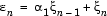 .
.AR(1) - The Autoregressive method has the form
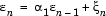 .
.AR(2) - The Autoregressive method of the form

 is a stochastic input,
  .
.