Stepwise Regression
Use the Stepwise functions to help fine a good model fit. The goal of the stepwise search is to minimize PRESS. Minimizing Predicted Error Sum of Squares (PRESS) is a good method for working toward a regression model that provides good predictive capability over the experimental factor space.
The use of PRESS is a key indicator of the predictive quality of a model. The predicted error uses predictions calculated without using the observed value for that observation. PRESS is known as Delete-1 statistics in the Statistics and Machine Learning Toolbox™ product.
You can choose automatic stepwise during model setup, or manual control using the Stepwise window.
Use the Stepwise menu in the Model Setup dialog boxes to run stepwise automatically when building linear models.
Open the stepwise regression window through the
 toolbar icon when you are in the global level
view. The Stepwise tool provides a number of methods of selecting the model
terms that should be included.
toolbar icon when you are in the global level
view. The Stepwise tool provides a number of methods of selecting the model
terms that should be included.
Automatic Stepwise
You can set the Minimize PRESS, Forward, and Backward selection routines to run automatically without the need to enter the stepwise figure.
You can set these options in the Model Setup dialog box, when you initially set up your test plan, or from the global level as follows:
Select Model > Set Up.
The Global Model Setup dialog box has a drop-down menu Stepwise, with the options
None,Minimize PRESS,Forward selection, andBackward selection.
Using the Stepwise Regression Window
Use the stepwise command buttons at the bottom of the window as follows:
Click Min. PRESS to automatically include or remove terms to minimize PRESS. This procedure provides a model with improved predictive capability.
Include All terms in the model (except the terms flagged with Status as
Never). This option is useful in conjunction with Min. PRESS and backward selection. For example, first click Include All, then Min. PRESS. Then you can click Include All again, then Backwards, to compare which gives the best result.Remove All terms in the model (except the terms flagged with Status as
Always). This option is useful in conjunction with forward selection (click Remove All, then Forwards).Forwards selection adds all terms to the model that would result in statistically significant terms at the ɑ% level (see Step 4 for alpha). The addition of terms is repeated until all the terms in the model are statistically significant.
Backwards selection removes all terms from the model that are not statistically significant at the ɑ% level. The removal of terms is repeated until all the terms in the model are statistically significant.
Terms can be also be manually included or removed from the model by clicking on the Term, Next PRESS, or coefficient error bar line.
The confidence intervals for all the coefficients are shown to the right of the table. Note that the interval for the constant term is not displayed, as the value of this coefficient is often significantly larger than other coefficients.
A history of the PRESS and summary statistics is shown on the right of the stepwise figure. You can return to a previous model by clicking an item in the list box or a point on the Stepwise PRESS History plot.
The critical values for testing whether a coefficient is statistically different from zero at the ɑ% level are displayed at the bottom right side of the stepwise figure. You can enter the value of ɑ% in the edit box (labeled 4 in the following figure) to the left of the critical values. The default is 5%. The ANOVA table is shown for the current model.
Any changes made in the stepwise figure automatically update the diagnostic plots in the Model Browser.
You can revert to the starting model when closing the Stepwise window. When you exit the
Stepwise window, the Confirm Stepwise Exit dialog box asks Do you want to
update regression results? You can click Yes,
No (to revert to the starting model), or
Cancel (to return to the Stepwise window).
Stepwise Table
| Term | Label for Coefficient |
|---|---|
Status | Always. Stepwise does not remove this term. Never. Stepwise does not add this term. Step. Stepwise considers this term for addition or removal. |
B | Value of coefficient. When the term is not in the model the value of the coefficient if it is added to the model is displayed in red. |
stdB | Standard error of coefficient. |
t | t value to test whether the coefficient is statistically different from zero. The t value is highlighted in blue if it is less than the critical value specified in the ɑ% edit box (at bottom right). |
Next PRESS | The value of PRESS if the inclusion or exclusion of this term is changed at the next iteration. A yellow highlighted cell indicates the next recommended term to change. Including or excluding the highlighted term (depending on its current state) will lead to the greatest reduction in the PRESS value. If there is no yellow highlighting this means that the PRESS value is already minimized. If there is a yellow cell, the column header is also yellow to alert you that you could make a change to achieve a smaller PRESS value. The column header is highlighted because you may need to scroll to find the yellow cell. |
The preceding table describes the meanings of the column headings in the Stepwise Regression window.
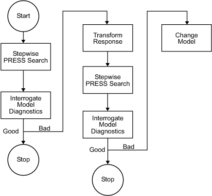
Stepwise in the Model Building Process
Once you have set up a model, you should create several alternative models, use the Stepwise functions and examine the diagnostic statistics to search for a good model fit. For each response feature,
Begin by conducting a stepwise search.
You can do this automatically or by using the Stepwise window.
The goal of the stepwise search is to minimize PRESS. Usually not one but several candidate models per response features arise, each with a very similar PRESS R2. The predictive capability of a model with a PRESS R2 of 0.91 cannot be assumed superior in any meaningful engineering sense to a model with a PRESS R2 of 0.909. Further, the nature of the model building process is that the "improvement" in PRESS R2 offered by the last few terms is often very small. Consequently, several candidate models can arise. You can store each of the candidate models and associated diagnostic information separately for subsequent review. Do this by making a selection of child nodes for the response feature.
However, experience has shown that a model with a PRESS R2 of less than 0.8, say, is of little use as a predictive tool for engine mapping purposes. This criterion must be viewed with caution. Low PRESS R2 values can result from a poor choice of the original factors but also from the presence of outlying or influential points in the data set. Rather than relying on PRESS R2 alone, a safer strategy is to study the model diagnostic information to discern the nature of any fundamental issues and then take appropriate corrective action.
Once the stepwise process is complete, the diagnostic data should be reviewed for each candidate model.
It might be that these data alone are sufficient to provide a means of selecting a single model. This would be the case if one model clearly exhibited more ideal behavior than the others. Remember that the interpretation of diagnostic plots is subjective.
You should also remove outlying data at this stage. You can set criteria for detecting outlying data. The default criterion is any case where the absolute value of the external studentized residual is greater than 3.
After removing outlying data, continue the model building process in an attempt to remove further terms.
High-order terms might have been retained in the model in an attempt to follow the outlying data. Even after removing outlying data, there is no guarantee that the diagnostic data will suggest that a suitable candidate model has been found. Under these circumstances,
A transform of the response feature might prove beneficial.
The Box and Cox family provides a useful set of transformations. Note that the Box-Cox algorithm is model dependent and as such is always carried out using the (Nxq) regression matrix
X.After you select a transform, you should repeat the stepwise PRESS search and select a suitable subset of candidate models.
After this you should analyze the respective diagnostic data for each model.
It might not be apparent why the original stepwise search was carried out in the natural metric. Why not proceed directly to taking a transformation? This seems sensible when it is appreciated that the Box-Cox algorithm often, but not always, suggests that a contractive transform such as the square root or log be applied. There are two main reasons for this:
The primary reason for selecting response features is that they possess a natural engineering interpretation. It is unlikely that the behavior of a transformed version of a response feature is as intuitively easy to understand.
Outlying data can strongly influence the type of transformation selected. Applying a transformation to allow the model to fit bad data well does not seem like a prudent strategy. By “bad” data it is assumed that the data is truly abnormal and a reason has been discovered as to why the data is outlying; for example, “The emission analyzer was purging while the results were taken.”
Finally, if you cannot find a suitable candidate model on completion of the stepwise search with the transformed metric, then a serious problem exists either with the data or with the current level of engineering knowledge of the system. Model augmentation or an alternative experimental or modeling strategy should be applied in these circumstances.
After these steps, validate your model against any other data.
This flow chart provides the recommended overall stepwise process.
Note
Carry out the process for each member of the set of response features associated with a given response. Then repeat the process for the remaining responses.
PRESS statistic
With n runs in the data set, the software fits the model equation to n-1 runs and a prediction taken from this model for the remaining one. The difference between the recorded data value and the value given by the model (at the value of the omitted run) is called a prediction residual. PRESS is the sum of squares of the prediction residuals. The square root of PRESS/n is PRESS RMSE (root mean square prediction error).
The prediction residual is different from the ordinary residual, which is the difference between the recorded value and the value of the model when fitted to the whole data set.
The PRESS statistic gives a good indication of the predictive power of your model, which is why minimizing PRESS is desirable. Comparing PRESS RMSE with RMSE may indicate problems with overfitting. RMSE is minimized when the model gets very close to each data point; 'chasing' the data will therefore improve RMSE. However, chasing the data can sometimes lead to strong oscillations in the model between the data points; this behavior can give good values of RMSE but is not representative of the data. It will not give reliable prediction values where you do not already have data. The PRESS RMSE statistic guards against this by testing how well the current model would predict each of the points in the data set (in turn) if they were not included in the regression. To get a small PRESS RMSE usually indicates that the model is not overly sensitive to any single data point.
Calculating PRESS for the two-stage model applies the same principle (fitting the model to n-1 runs and taking a prediction from this model for the remaining one). However, the predicted values are first found for response features instead of data points. The predicted value, omitting each test in turn, for each response feature is estimated. The predicted response features are then used to reconstruct the local curve for the test and this curve is used to obtain the two-stage predictions. This is applied as follows:
To calculate two stage PRESS:
For each test, S, do the following steps:
For each of the response features, calculate what the response feature predictions would be for S (with the response features for S removed from the calculation).
This gives a local prediction curve C based on all tests except S.
For each data point in the test, calculate the difference between the observed value and the value predicted by C.
Repeat for all tests.
Sum the square of all of the differences found and divide by the total number of data points.