Determine Reference Currents for PMSM Using Characterization Test Data

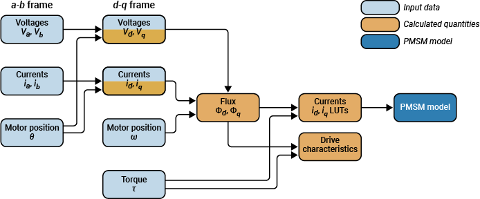
This example uses:

This example shows how to determine the drive characteristics and optimal reference currents for a non-linear permanent magnet synchronous motor (PMSM) from measured or simulated test data. It computes lookup tables (LUTs) for $d$ and $q$ axis reference currents $i_{d}$ and $i_{q}$ as a function of motor speed and load torque. A plant model loads the calculated LUTs and simulates the motor dynamics.

Prerequisites

To calculate the optimal reference currents, this example requires input voltage, current, motor speed, and torque data. Provide data from physical measurements (such as from dyno tests) or virtual dyno FEA simulations.

Import Non-Linear Motor Data from Dyno Tests or FEA Tools

Import the following non-linear motor data.

Voltages along $a$ and $b$ axes, $V_{a}$ and $V_{b}$ or $d$ and $q$ axes, $V_{d}$ and $V_{q}$ (V)
Currents along $a$ and $b$ axes, $i_{a}$ and $i_{b}$ or $d$ and $q$ axes, $i_{d}$ and $i_{q}$ (A)
Motor speed, $ω$ (rpm)
Torque, $T$ (N.m)

You can choose to import data from the following sources.

Physical measurements in the stationary ( $a$ - $b$ ) frame. This script calculates the corresponding values in the rotor ( $d$ - $q$ ) frame from the provided motor position $θ$ using Clarke and Park transforms.
Physical measurements in the rotor ( $d$ - $q$ ) frame
FEA based virtual dyno simulation. Select this option if you do not have preexisting data to import. This script loads data from the pmsmData_LdLq.mat and DynoData.mat data files.
FEA simulation sample data

Specify how to import data by selecting an option from the data_input_type menu. Each option corresponds to a case and the code below it. For the first three options, this script calculates the fluxes along $d$ and $q$ axes $Φ_{d}$ and $Φ_{q}$ (Wb) from the imported data. For the last option, you must provide the flux data.

data_input_type=3;

switch(data_input_type)
    case 1
        % Capture voltages, currents, position, speed and torque
        % from the signals from the system
        Test_data=[% va, vb, ia, ib, theta_m, w_rpm, T_Nm
            ];
        va=Test_data(:,1);
        vb=Test_data(:,2);
        ia=Test_data(:,3);
        ib=Test_data(:,4);
        theta_m=Test_data(:,5);
        w_rpm=Test_data(:,6);
        wm_radps=w_rpm*pi/30;
        T_Nm=Test_data(:,7);
        vd=cos(theta_m*pp).*va+sin(theta_m*pp).*(va+vb*2)/sqrt(3);
        vq=-sin(theta_m*pp).*va+cos(theta_m*pp).*(va+2*vb)/sqrt(3);
        id=cos(theta_m*pp).*ia+sin(theta_m*pp).*(ia+ib*2)/sqrt(3);
        iq=-sin(theta_m*pp).*ia+cos(theta_m*pp).*(ia+2*ib)/sqrt(3);
        fluxQ=(id*pmsm.Rs-vd)./(pmsm.p*wm_radps);
        fluxD=(vq-iq*pmsm.Rs)./(pmsm.p*wm_radps);
    case 2
        % Capture voltages and currents from dq axes of reference,
        % along with speed and torque
        Test_data=[% vd vq id iq wm_radps T_Nm
            ];
        vd=Test_data(:,1);
        vq=Test_data(:,2);
        id=Test_data(:,3);
        iq=Test_data(:,4);
        w_rpm=Test_data(:,5);
        wm_radps=w_rpm*pi/30;
        T_Nm=Test_data(:,6);
        fluxQ=(id*pmsm.Rs-vd)./(pmsm.p*wm_radps);
        fluxD=(vq-iq*pmsm.Rs)./(pmsm.p*wm_radps);
    case 3
        % Virtual dyno simulation based on the FEA simulation data
        load('pmsmData_LdLq.mat');
        pmsm.PMSMLUT=PMSMLUT;
        pmsm.PMSMLUT.method='Ldq';
        PU_System = mcb.getPUSystemParameters(pmsm,inverter);
        load('DynoData.mat'); % this data file is from virtual dyno simulation (using PU system).
        Final_data=DynoData;
        vd=Final_data(:,1)*PU_System.V_base;
        vq=Final_data(:,2)*PU_System.V_base;
        id=Final_data(:,3)*PU_System.I_base;
        iq=Final_data(:,4)*PU_System.I_base;
        wm_radps=Final_data(:,5);
        T_Nm=Final_data(:,6);
        fluxQ=(id*pmsm.Rs-vd)./(pmsm.p*wm_radps);
        fluxD=(vq-iq*pmsm.Rs)./(pmsm.p*wm_radps);
        w_rpm=wm_radps*30/pi;
    case 4
        % FEA simulation sample data 
        Test_data=[id iq fluxD fluxQ w_rpm T_Nm;
            ];
end

Additionally, input operating parameters for the motor and inverter.

I_rated     =   PU_System.I_base;       % A
Vdc         =   inverter.V_dc;
pp          =   pmsm.p;                 % number of pole pairs
Rs          =   pmsm.Rs;                % Ohm 
clf;

Compute Surface Maps for Flux and Torque

Process the input data to generate grid spaces for the currents, and surface maps for the flux and torque.

Define the grid spaces for currents for characterization and automatically create surface maps.

idAxis = linspace(-I_rated,0,50);
iqAxis = linspace(0,I_rated,51);
[IDgrid,IQgrid] = ndgrid(idAxis,iqAxis);
currentBreakpoints = {idAxis,iqAxis};
lambdad = fitlookupn(currentBreakpoints,[id,iq],fluxD,8,ShowPlot=1);
title("Flux d [Wb]");
xlabel("Id [A]");
ylabel("Iq [A]");

Figure contains an axes object. The axes object with title Flux d [Wb], xlabel Id [A], ylabel Iq [A] contains 3 objects of type surface, line. One or more of the lines displays its values using only markers

lambdaq = fitlookupn(currentBreakpoints,[id,iq],fluxQ,5,ShowPlot=1);
title("Flux q [Wb]");
xlabel("Id [A]");
ylabel("Iq [A]");

Figure contains an axes object. The axes object with title Flux q [Wb], xlabel Id [A], ylabel Iq [A] contains 3 objects of type surface, line. One or more of the lines displays its values using only markers

torque = fitlookupn(currentBreakpoints,[id,iq],T_Nm,5,ShowPlot=1);
title("Torque [Wb]");
xlabel("Id [A]");
ylabel("Iq [A]");

Figure contains an axes object. The axes object with title Torque [Wb], xlabel Id [A], ylabel Iq [A] contains 3 objects of type surface, line. One or more of the lines displays its values using only markers

Find Drive Characteristics and Generate Optimal Reference Current LUTs

Define Speed and Torque Grid

Define the speed and torque breakpoints over which to generate the reference id and iq current LUTs.

The maximum speed and torque values cover the maximum values achievable in this example PMSM application. Adjust these values to suit the range of speeds and torques appropriate for your motor setup and simulation needs.

Additionally, adjust the number of grid points ngridpts along each dimension. More grid points improves the accuracy of nonlinearity tracing for LUT generation, but incurs more costs in terms of memory and computation speed.

pmsm.Rs=Rs;
pmsm.p=pp;
pmsm.I_rated=I_rated;
pmsm.B=1e-6;
pmsm.J=1e-6;

ngridpts = 40;
RPMGrid = [100 linspace( 500, min(25000,mcb.PMSMMaxSpeed(pmsm,inverter)), ngridpts)];
TrqMax = max(abs(torque),[],"all");
NmGrid  = [0 0.1 linspace(0.5,min(TrqMax,mcb.PMSMRatedTorque(pmsm,inverter)), ngridpts)];

Load Motor Parameters

Load the motor parameters into the pmsm and inverter data structures.

[id_m1,iq_m1]=meshgrid(idAxis,iqAxis);
pmsm.PMSMLUT.idVec=idAxis;
pmsm.PMSMLUT.iqVec=iqAxis;
pmsm.PMSMLUT.FluxDTable=lambdad;
pmsm.PMSMLUT.FluxQTable=lambdaq;
pmsm.PMSMLUT.method='FluxDQ';
pmsm.PMSMLUT.TorqueTable=torque;
pmsm.PMSMLUT.wrpmVec=double(RPMGrid);
pmsm.PMSMLUT.trefVec=NmGrid;
pmsm.PMSMLUT.motorType='ipmsm';
pmsm.motorType='ipmsm';
inverter.V_dc=Vdc;

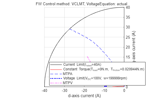
Plot Constraint Curves and Drive Characteristics

Determine PMSM constraint curves from the processed data, and plot the associated drive characteristics. For more information about synchronous motor constraint curves and drive characteristics, see these topics:

mcb.PMSMCharacteristics(pmsm,inverter,constraintCurves=1);

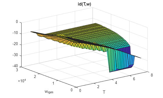
$Figure Constraint Curves of pmsm contains an axes object and another object of type subplottext. The axes object with xlabel d-axis current (A), ylabel q-axis current (A) contains 5 objects of type line. These objects represent Current Limit(I_{rated}=40A), Constant Torque(T_{load}=0N.m, T_{friction}=0.020944N.m), MTPA, Voltage Limit(V_{DC}=100V, w=199999rpm), MTPV.$

Compute and Plot Optimal Reference Currents

Compute optimal reference current LUTs PMSMLUT.idTable and PMSMLUT.iqTable, then create surface maps of these currents. For more information about the generation of optimal reference currents, see Plot Constraint Curves and Drive Characteristics for PMSM and SynRM Directly from Block Parameters Dialog Box.

PMSMLUT=mcb.generateMotorLUT(pmsm,inverter,'idiqluts',useTorquePercent=0,drawLUT=1);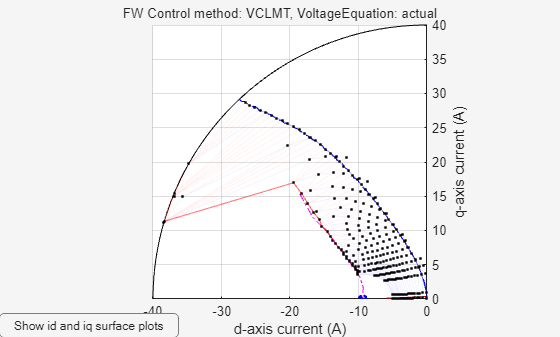

$Figure Constraint Curves of pmsm contains an axes object and other objects of type subplottext, uicontrol. The axes object with xlabel d-axis current (A), ylabel q-axis current (A) contains 88 objects of type line. These objects represent Current Limit(I_{rated}=40A), Constant Torque(T_{load}=0N.m, T_{friction}=0.020944N.m), MTPA, Voltage Limit(V_{DC}=100V, w=199999rpm), MTPV.$

figure;surf(PMSMLUT.trefVec,PMSMLUT.wrpmVec,PMSMLUT.idTable');xlabel('T');ylabel('w_{rpm}');title('id(T,w)');

Figure contains an axes object. The axes object with title id(T,w), xlabel T, ylabel w indexOf rpm baseline contains an object of type surface.

figure;surf(PMSMLUT.trefVec,PMSMLUT.wrpmVec,PMSMLUT.iqTable');xlabel('T');ylabel('w_{rpm}');title('iq(T,w)');

Figure contains an axes object. The axes object with title iq(T,w), xlabel T, ylabel w indexOf rpm baseline contains an object of type surface.

Prepare and Simulate Model

Create a new model containing a LUT based PMSM Control Reference block, which uses iterative methods and specified LUTs to calculate reference currents along the d-q axes. Specify block parameters such as Reference id LUT, id(Tref,wrpm) (A) and Reference iq LUT, id(Tref,wrpm) (A).

Alternatively, open the prepopulated model RunNonlinearPMSM.

model_type = 2;

switch(model_type)
    case 1
        open_system(new_system);
        add_block('mcbpmsmnonlinearlib/LUT based PMSM Control Reference','untitled/IPMSM');
        set_param('untitled/IPMSM','polePairs','pmsm.p');
        set_param('untitled/IPMSM','Rs','pmsm.Rs');
        set_param('untitled/IPMSM','nonLinearityChoice','Non-linear model with id and iq LUTs');
        set_param('untitled/IPMSM','vdc','inverter.V_dc');
        set_param('untitled/IPMSM','trefVec','PMSMLUT.trefVec','wrpmVec','PMSMLUT.wrpmVec','idTable','PMSMLUT.idTable','iqTable','PMSMLUT.iqTable','ilimit','pmsm.I_rated','Bv','pmsm.B');
        set_param('untitled/IPMSM','Units','SI Units');
    case 2
        mlx_done=1;
        pmsm.PMSMLUT=PMSMLUT;
        open("RunNonlinearPMSM.slx");
end

This model simulates the dynamics of a nonlinear PMSM operating under FOC at a specified motor speed and load torque. In the Control System subsystem, the Torque Control subsystem contains a LUT based PMSM Control Reference block.

For either model, in the Block Parameters dialog box for the LUT based PMSM Control Reference block, verify that Motor parameter input method is set to Non-linear model with id and iq LUTs and that Reference id LUT, id(Tref,wrpm) (A) and Reference iq LUT, id(Tref,wrpm) (A) are set to PMSMLUT.idTable and PMSMLUT.iqTable, respectively.

If you selected model RunNonlinearPMSM, the block outputs the $d$ -axis and $q$ -axis reference currents from the input motor speed, load torque, and battery voltage. The torque control system then compares the computed reference currents against measured currents to determine reference voltages and PWM duty cycles.