Model Predictive Control of Multi-Input Single-Output Plant

Define Plant Model

Define a plant model. For this example, use continuous-time transfer functions from each input to the output.

plantTF = tf({1,1,1},{[1 .5 1],[1 1],[.7 .5 1]}) % define and display tf object

plantTF =
 
  From input 1 to output:
         1
  ---------------
  s^2 + 0.5 s + 1
 
  From input 2 to output:
    1
  -----
  s + 1
 
  From input 3 to output:
           1
  -------------------
  0.7 s^2 + 0.5 s + 1
 
Continuous-time transfer function.

For this example, explicitly convert the plant to a discrete-time state-space form before passing it to the MPC controller creation function.

The controller creation function can accept either continuous-time or discrete-time plants. During initialization, a continuous-time plant (in any format) is automatically converted into a discrete-time state-space model using the zero-order hold (ZOH) method. Delays, if present, are incorporated in the state-space model.

You can convert the plant to discrete-time yourself when you need the discrete-time system matrices for analysis or simulation (as in this example) or when you want to use a discrete-time conversion method other than ZOH.

plantCSS = ss(plantTF);         % transfer function to continuous state space
Ts = 0.2;                       % specify a sample time of 0.2 seconds
plantDSS = c2d(plantCSS,Ts)     % convert to discrete-time state space, using ZOH

plantDSS =
 
  A = 
            x1       x2       x3       x4       x5
   x1   0.8862  -0.1891        0        0        0
   x2   0.1891   0.9807        0        0        0
   x3        0        0   0.8187        0        0
   x4        0        0        0    0.841  -0.2637
   x5        0        0        0   0.1846   0.9729
 
  B = 
            u1       u2       u3
   x1   0.1891        0        0
   x2  0.01929        0        0
   x3        0   0.1813        0
   x4        0        0   0.1846
   x5        0        0  0.01899
 
  C = 
          x1     x2     x3     x4     x5
   y1      0      1      1      0  1.429
 
  D = 
       u1  u2  u3
   y1   0   0   0
 
Sample time: 0.2 seconds
Discrete-time state-space model.

By default, the software assumes that all the plant input signals are manipulated variables. To specify the signal types, such as measured and unmeasured disturbances, use the setmpcsignals function. In this example, the first input signal is a manipulated variable, the second is a measured disturbance, and the third is an unmeasured disturbance. This information is stored in the plant model plantDSS and later used by the MPC controller.

plantDSS = setmpcsignals(plantDSS,'MV',1,'MD',2,'UD',3); % specify signal types

Design MPC Controller

Create the controller object, specifying the sample time, as well as the prediction and control horizons (10 and 3 steps, respectively).

mpcobj = mpc(plantDSS,Ts,10,3);

-->"Weights.ManipulatedVariables" is empty. Assuming default 0.00000.
-->"Weights.ManipulatedVariablesRate" is empty. Assuming default 0.10000.
-->"Weights.OutputVariables" is empty. Assuming default 1.00000.

Since you have not specified the weights of the quadratic cost function to be minimized, the controller uses their default values (0 for manipulated variables, 0.1 for manipulated variable rates, and 1 for the output variables). Also, at this point the MPC problem is still unconstrained as you have not specified any constraint yet.

Define hard constraints on the manipulated variable.

mpcobj.MV = struct('Min',0,'Max',1,'RateMin',-10,'RateMax',10);

You can use input and output disturbance models to define the dynamic characteristics of additive input and output unmeasured disturbances. These models allow the controller to better reject such disturbances, if they occur at run time. By default, to be able to better reject step-like disturbances, mpc uses an integrator as disturbance model for:

unless doing so causes a violation of state observability.

The MPC object also has a noise model that specifies the characteristics of the additive noise that is expected on the measured output variables. By default, this is assumed to be a unit static gain, which is equivalent to assuming that the controller expects the measured output variables to be affected, at run time, by white noise (with a covariance matrix that depends on the input matrices of the whole prediction model). For more information, see MPC Prediction Models.

Display the input disturbance model. As expected, it is a discrete-time integrator.

getindist(mpcobj)

-->The "Model.Disturbance" property is empty:
   Assuming unmeasured input disturbance #3 is integrated white noise.
   Assuming no disturbance added to measured output #1.
-->"Model.Noise" is empty. Assuming white noise on each measured output.

ans =
 
  A = 
       x1
   x1   1
 
  B = 
       UD1-wn
   x1     0.2
 
  C = 
        x1
   UD1   1
 
  D = 
        UD1-wn
   UD1       0
 
Sample time: 0.2 seconds
Discrete-time state-space model.

Display the output disturbance model.

getoutdist(mpcobj)

ans =

  Empty state-space model.

Specify the disturbance model for the unmeasured input as an integrator driven by white noise with variance 1000.

mpcobj.Model.Disturbance = tf(sqrt(1000),[1 0]);

Display the input disturbance model again to verify that it changed.

getindist(mpcobj)

ans =
 
  A = 
       x1
   x1   1
 
  B = 
       Noise#1
   x1      0.8
 
  C = 
           x1
   UD1  7.906
 
  D = 
        Noise#1
   UD1        0
 
Sample time: 0.2 seconds
Discrete-time state-space model.

Display the MPC controller object mpcobj to review its properties.

mpcobj

 
MPC object (created on 05-Sep-2024 14:43:20):
---------------------------------------------
Sampling time:      0.2 (seconds)
Prediction Horizon: 10
Control Horizon:    3

Plant Model:        
                                      --------------
      1  manipulated variable(s)   -->|  5 states  |
                                      |            |-->  1 measured output(s)
      1  measured disturbance(s)   -->|  3 inputs  |
                                      |            |-->  0 unmeasured output(s)
      1  unmeasured disturbance(s) -->|  1 outputs |
                                      --------------
Indices:
  (input vector)    Manipulated variables: [1 ]
                    Measured disturbances: [2 ]
                  Unmeasured disturbances: [3 ]
  (output vector)        Measured outputs: [1 ]

Disturbance and Noise Models:
        Output disturbance model: default (type "getoutdist(mpcobj)" for details)
         Input disturbance model: user specified (type "getindist(mpcobj)" for more details)
         Measurement noise model: default (unity gain after scaling)

Weights:
        ManipulatedVariables: 0
    ManipulatedVariablesRate: 0.1000
             OutputVariables: 1
                         ECR: 100000

State Estimation:  Default Kalman Filter (type "getEstimator(mpcobj)" for details)

Constraints:
 0 <= MV1 <= 1, -10 <= MV1/rate <= 10, MO1 is unconstrained

Use built-in "active-set" QP solver with MaxIterations of 120.

Examine Steady-State Offset

To examine whether the MPC controller can reject constant output disturbances and track a constant setpoint with zero offsets in steady state, calculate the closed-loop DC gain from output disturbances to controlled outputs using the cloffset command. This gain is also known as the steady state output sensitivity of the closed loop.

DC = cloffset(mpcobj);
fprintf('DC gain from output disturbance to output = %5.8f (=%g) \n',DC,DC);

   Assuming no disturbance added to measured output #1.
-->"Model.Noise" is empty. Assuming white noise on each measured output.
DC gain from output disturbance to output = 0.00000000 (=2.77556e-15) 

A zero gain, which is typically the result of the controller having integrators as input or output disturbance models, means that the measured plant output tracks the desired output reference setpoint perfectly in steady state.

Simulate Closed-Loop Response Using sim

The sim command provides a quick way to simulate an MPC controller in a closed loop with a linear time-invariant plant when constraints and weights stay constant and you can easily and completely specify the disturbance and reference signals ahead of time.

First, specify the simulation time and the reference and disturbance signals

Tstop = 30;                               % simulation time
Nf = round(Tstop/Ts);                     % number of simulation steps
r = ones(Nf,1);                           % output reference signal
v = [zeros(Nf/3,1);ones(2*Nf/3,1)];       % measured input disturbance signal

Run the closed-loop simulation and plot the results. The plant specified in mpcobj.Model.Plant is used both as the plant in the closed-loop simulation and as the internal plant model used by the controller to predict the response over the prediction horizon. The plant model is discretized or resampled if needed, and the simulation runs in discrete time, with sample time mpcobj.Ts.

Use sim to simulate the closed-loop response to reference r and measured input disturbance v system for Nf steps.

sim(mpcobj,Nf,r,v)      % simulate plant and controller in closed loop

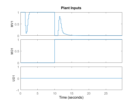
The manipulated variable hits the upper bound initially, and brings the plant output to the reference value within a few seconds. The manipulated variable then settles at its maximum allowed value, 1. After 10 seconds, the measured disturbance signal rises from 0 to 1, which causes the plant output to exceed its reference value by about 30%. The manipulated variable hits the lower bound in an effort to reject the disturbance. The controller is able to bring the plant output back to the reference value after a few seconds, and the manipulated variable settles at its minimum value. The unmeasured disturbance signal is always zero, because no unmeasured disturbance signal has been specified yet.

You can use a simulation options object to specify additional simulation options and additional signals, such as noise and unmeasured disturbances, that feed into the plant but are unknown to the controller. For this example, use a simulation option object to add an unmeasured input disturbance signal to the manipulated variable and to add noise on the measured output signal. Create a simulation options object with default options.

SimOptions = mpcsimopt;                       % create object

Create a disturbance signal and specify it in the simulation options object.

d = [zeros(2*Nf/3,1);-0.5*ones(Nf/3,1)];      % step disturbance
SimOptions.UnmeasuredDisturbance = d;         % unmeasured input disturbance

Specify noise signals in the simulation options object. At simulation time, the simulation function directly adds the specified output noise to the measured output before feeding it to the controller. It also directly adds the specified input noise to the manipulated variable (not to any disturbance signals) before feeding it to the plant.

SimOptions.OutputNoise=.001*(rand(Nf,1)-.5);  % output measurement noise
SimOptions.InputNoise=.05*(rand(Nf,1)-.5);    % noise on manipulated variables

You can also use the OutputNoise field of the simulation option object to specify a more general additive output disturbance signal (such as a step) on the measured plant output.

Simulate the closed-loop system and save the results to the workspace variables y, t, u, and xp. Saving this variables allows you to selectively plot signals in a new figure window and in any given color and order.

[y,t,u,xp] = sim(mpcobj,Nf,r,v,SimOptions);

Plot the results.

figure                                  % create new figure

subplot(2,1,1)                          % create upper subplot
plot(0:Nf-1,y,0:Nf-1,r)                 % plot plant output and reference
title('Output')                         % add title so upper subplot
ylabel('MO1')                           % add a label to the upper y axis
grid                                    % add a grid to upper subplot

subplot(2,1,2)                          % create lower subplot
plot(0:Nf-1,u)                          % plot manipulated variable
title('Input');                         % add title so lower subplot
xlabel('Simulation Steps')              % add a label to the lower x axis
ylabel('MV1')                           % add a label to the lower y axis
grid                                    % add a grid to lower subplot

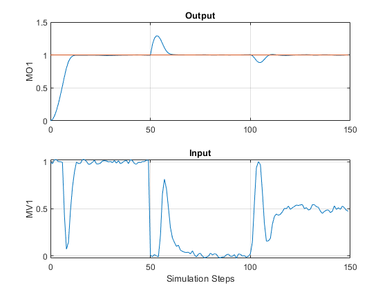
Despite the added noise, which is especially visible on the manipulated variable plot, and despite the measured and unmeasured disturbances starting after 50 and 100 steps, respectively, the controller is able to achieve good tracking. The manipulated variable settles at about 1 after the initial part of the simulation (steps from 20 to 50), at about 0 to reject the measured disturbance (steps from 70 to 100), and at about 0.5 to reject both disturbances (steps from 120 to 150).

Simulate Closed-Loop Response with Model Mismatch

Test the robustness of the MPC controller against a model mismatch. Specify the true plant that you want to use in simulation as truePlantCSS. For this example, the denominator of each of the three plant transfer functions has one or two coefficients that differ from the corresponding ones in the plant defined earlier in Define Plant model section, which the MPC controller uses for prediction.

truePlantTF = tf({1,1,1},{[1 .8 1],[1 2],[.6 .6 1]})    % specify and display transfer functions
truePlantCSS = ss(truePlantTF);                         % convert to continuous state space
truePlantCSS = setmpcsignals(truePlantCSS,'MV',1,'MD',2,'UD',3); % specify signal types

truePlantTF =
 
  From input 1 to output:
         1
  ---------------
  s^2 + 0.8 s + 1
 
  From input 2 to output:
    1
  -----
  s + 2
 
  From input 3 to output:
           1
  -------------------
  0.6 s^2 + 0.6 s + 1
 
Continuous-time transfer function.

Update the simulation option object by specifying SimOptions.Model as a structure with two fields, Plant (containing the true plant model) and Nominal (containing the operating point values for the true plant). For this example, the nominal values for the state derivatives and the inputs are not specified, so they are assumed to be zero, resulting in y = SimOptions.Model.Nominal.Y + C*(x-SimOptions.Model.Nominal.X), where x and y are the state and measured output of the plant, respectively.

% create the structure and assign the 'Plant' field
SimOptions.Model = struct('Plant',truePlantCSS);

 % create and assign the 'Nominal.Y' field
SimOptions.Model.Nominal.Y = 0.1;

% create and assign the 'Nominal.X' field
SimOptions.Model.Nominal.X = -.1*[1 1 1 1 1];

% specify the initial state of the true plant
SimOptions.PlantInitialState = [0.1 0 -0.1 0 .05];

Remove any signal that have been added to the measured output and to the manipulated variable.

SimOptions.OutputNoise = [];            % remove output measurement noise
SimOptions.InputNoise = [];             % remove noise on manipulated variable

Run the closed-loop simulation and plot the results. Since SimOptions.Model is not empty, SimOptions.Model.Plant is converted to discrete time (using zero order hold) and used as the plant in the closed loop simulation, while the plant in mpcobj.Model.Plant is only used by the controller to predict the response over the prediction horizon.

sim(mpcobj,Nf,r,v,SimOptions)           % simulate the closed loop

-->Converting model to discrete time.

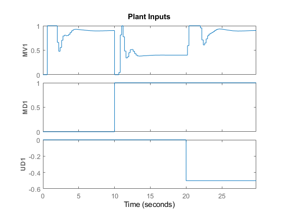
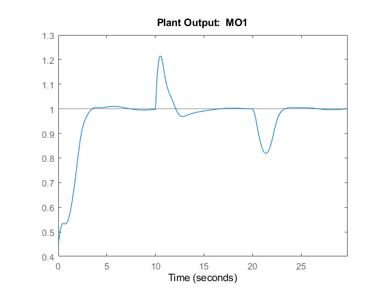
As a result of the model mismatch, some degradation in the response is visible; notably, the controller needs a little more time to achieve tracking and the manipulated variable now settles at about 0.5 to reject the measured disturbance (see values from 5 to 10 seconds) and settles at about 0.9 to reject both input disturbances (from 25 to 30 seconds). Despite this degradation, the controller is still able to track the output reference.

Simulate Open-Loop Response

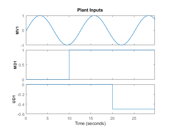
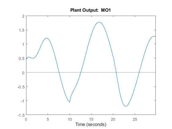
You can also test the behavior of the plant and controller in open-loop, using the sim command. Set the OpenLoop flag to on, and provide a sequence of manipulated variable values to excite the system (the sequence is ignored if OpenLoop is set to off).

SimOptions.OpenLoop = 'on';                 % set open loop option
SimOptions.MVSignal = sin((0:Nf-1)'/10);    % define mv signal

Simulate the true plant (previously specified in SimOptions.Model) in open loop. Since the reference signal is ignored in an open-loop simulation specify it as [].

sim(mpcobj,Nf,[],v,SimOptions)              % simulate the open loop system

-->Converting model to discrete time.

Soften Constraints

For an MPC controller, each constraint has an associated dimensionless ECR value. A constraint with a larger ECR value is allowed to be violated more than a constraint with a smaller ECR value. By default all constraints on the manipulated variables have an ECR value of zero, making them hard. You can specify a nonzero ECR value for a constraint to make it soft.

Relax the constraints on manipulated variables from hard to soft.

mpcobj.ManipulatedVariables.MinECR = 1;   % ECR for the MV lower bound
mpcobj.ManipulatedVariables.MaxECR = 1;   % ECR for the MV upped bound

Define an output constraint. By default all constraints on output variables (measured outputs) have an ECR value of one, making them soft. You can reduce the ECR value for an output constraint to make it harder, however best practice is to keep output constraints soft. Soft output constraints are preferred because plant outputs depend on both plant states and measured disturbances; therefore, if a large enough disturbance occurs, the plant outputs constraints can be violated regardless of the plant state (and therefore regardless of any control action taken by the MPC controller). These violations are especially likely when the manipulated variables have hard constraints. Such an unavoidable violation of a hard constraint results in an infeasible MPC problem, for which no manipulated variable can be calculated.

mpcobj.OutputVariables.Max = 1.1;    % define the (soft) output constraint

Run a new closed-loop simulation, without including the simulation option object, and therefore without any model mismatch, unmeasured disturbance, or noise added to the manipulated variable or measured output.

sim(mpcobj,Nf,r,v)          % simulate the closed loop

   Assuming no disturbance added to measured output #1.
-->"Model.Noise" is empty. Assuming white noise on each measured output.

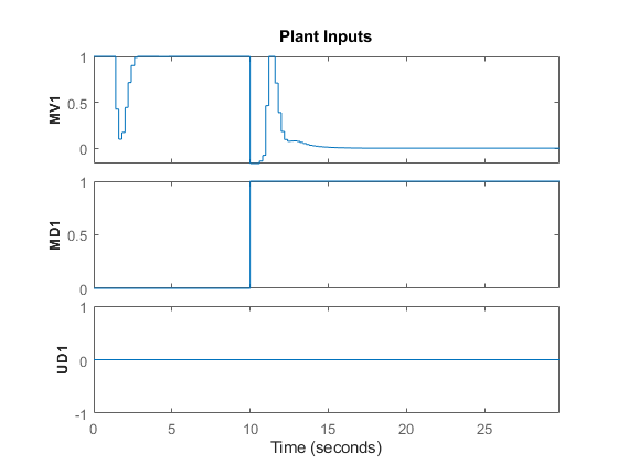
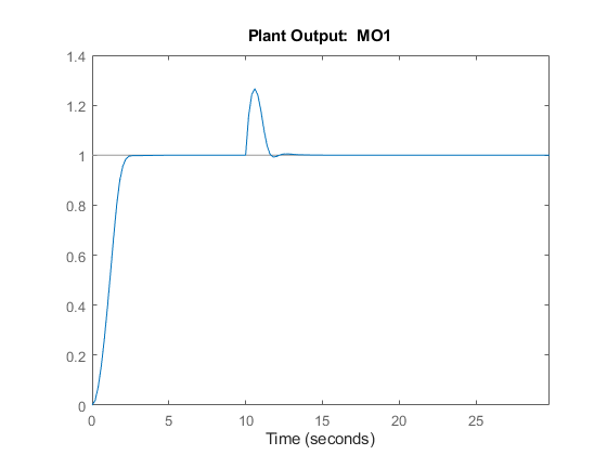
In an effort to reject the measured disturbance, achieve tracking, and prevent the output from rising above its soft constraint of 1.1, the controller slightly violates the soft constraint on the manipulated variable, which reaches small negative values from seconds 10 to 11. The controller violates the constraint on the measured output more than the constraint on the manipulated variable.

Harden the constraint on the output variable and rerun the simulation.

mpcobj.OV.MaxECR = 0.001;   % the closer to zero, the harder the constraint
sim(mpcobj,Nf,r,v)          % run a new closed-loop simulation.

   Assuming no disturbance added to measured output #1.
-->"Model.Noise" is empty. Assuming white noise on each measured output.

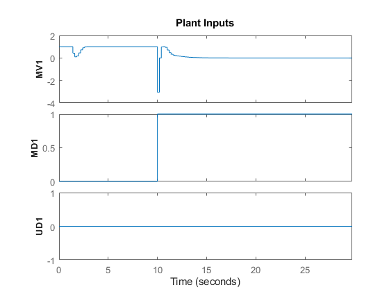
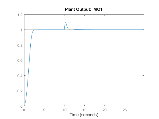
Now the controller violates the output constraint only slightly. This output performance improvement comes at the cost of violating the manipulated variable constraint a lot more (the manipulated variable reaches a value of -3).

Change Built-In State Estimator Kalman Gains

At each time step, the MPC controller computes the manipulated variable by solving a constrained quadratic optimization problem that depends on the current state of the plant. Since the plant state is often not directly measurable, by default, the controller uses a linear Kalman filter as an observer to estimate the state of the plant and the disturbance and noise models. Therefore, the states of the controller are the states of this Kalman filter, which are in turn the estimates of the states of the augmented discrete-time plant. Run a closed-loop simulation with model mismatch and unmeasured disturbance, using the default estimator, and return the controller state structure xc.

SimOptions.OpenLoop = 'off';                    % set closed loop option
[y,t,u,xp,xc] = sim(mpcobj,Nf,r,v,SimOptions);  % run simulation

-->In closed-loop simulation, the "MVSignal" property of "mpcsimopt" object is ignored.
-->Converting model to discrete time.

xc

xc = 

  struct with fields:

          Plant: [150x5 double]
    Disturbance: [150x1 double]
          Noise: [150x0 double]
       LastMove: [150x1 double]

Plot the plant output response as well as the plant states that have been estimated by the default observer.

figure;                                     % create figure

subplot(2,1,1)                              % create upper subplot axis
plot(t,y)                                   % plot y versus time
title('Plant Output');                      % add title to upper plot
ylabel('y')                                 % add a label to the upper y axis
grid                                        % add grid to upper plot

subplot(2,1,2)                              % create lower subplot axis
plot(t,xc.Plant)                            % plot xc.Plant versus time
title('Estimated Plant States');            % add title to lower plot
xlabel('Time (seconds)')                    % add a label to the lower x axis
ylabel('xc')                                % add a label to the lower y axis
grid                                        % add grid to lower plot

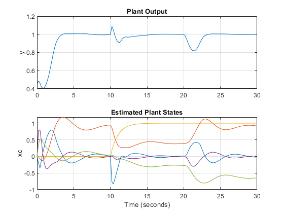
As expected, the measured and unmeasured disturbances cause sudden changes at 10 and 20 seconds, respectively.

You can change the gains of the Kalman filter. To do so, first, retrieve the default Kalman gains and state-space matrices.

[L,M,A1,Cm1] = getEstimator(mpcobj);    % retrieve observer matrices

Calculate and display the poles of the default observer. They are all inside the unit circle, though a few of them seem to be relatively close to the border. Note the six states, the first five belonging to the plant model and the sixth belonging to the input disturbance model.

e = eig(A1-A1*M*Cm1)                    % eigenvalues of observer state matrix

e =

   0.5708 + 0.4144i
   0.5708 - 0.4144i
   0.4967 + 0.0000i
   0.9334 + 0.1831i
   0.9334 - 0.1831i
   0.8189 + 0.0000i

Design a new state estimator using pole placement. Move the faster poles a little toward the origin and the slowest a little away from the origin. Everything else being equal, this pole placement should result in a slightly slower observer.

poles = [.8 .75 .7 .85 .6 .81]; % specify desired positions for the new poles
L = place(A1',Cm1',poles)';     % calculate Kalman gain for time update
M = A1\L;                       % calculate Kalman gain for measurement update

Set the new matrix gains in the MPC controller object.

setEstimator(mpcobj,L,M);               % set the new estimation gains

Rerun the closed-loop simulation.

[y,t,u,xp,xc] = sim(mpcobj,Nf,r,v,SimOptions);

   Assuming no disturbance added to measured output #1.
-->"Model.Noise" is empty. Assuming white noise on each measured output.
-->In closed-loop simulation, the "MVSignal" property of "mpcsimopt" object is ignored.
-->Converting model to discrete time.

Plot the plant output response as well as the plant states estimated by the new observer.

figure;                                     % create figure

subplot(2,1,1)                              % create upper subplot axis
plot(t,y)                                   % plot y versus time
title('Plant Output');                      % add title to upper plot
ylabel('y')                                 % add a label to the upper y axis
grid                                        % add grid to upper plot

subplot(2,1,2)                              % create lower subplot axis
plot(t,xc.Plant)                            % plot xc.Plant versus time
title('Estimated Plant States');            % add title to lower plot
xlabel('Time (seconds)')                    % add a label to the lower x axis
ylabel('xc')                                % add a label to the lower y axis
grid                                        % add grid to lower plot

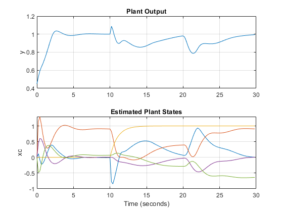
As expected, the controller states are different from the ones previously plotted, and the overall closed-loop response is somewhat slower.

Simulate Controller in Closed Loop Using mpcmove

For more general applications, you can simulate an MPC controller in a for loop using the mpcmove function. Using this function, you can run simulations with the following features.

If your plant is continuous, you can either convert it to discrete time before simulating or you can use a numerical integration algorithm (such as forward Euler or ode45) to simulate it in a closed loop using mpcmove. For example, you can calculate the plant state at the next control interval using the following methods:

In the third case, ode45 starts from the initial condition x and simulates the plant for Ts seconds, under a constant control signal u. The last value of the resulting state signal xhist is the plant state at the next control interval.

First, obtain the discrete-time state-space matrices of the plant, and define the simulation time and initial states for plant and controller.

[A,B,C,D] = ssdata(plantDSS);       % discrete-time plant plant ss matrices
Tstop = 30;                         % simulation time
x = [0 0 0 0 0]';                   % initial state of the plant
xmpc = mpcstate(mpcobj);            % get handle to controller state
r = 1;                              % output reference signal

Display the initial state of the controller. The state, which is an mpcstate object, contains the controller states only at the current time. Specifically: * |xmpc.Plant| is the current value of the estimated plant states. * |xmpc.Disturbance| is the current value of the disturbance models states. * |xmpc.Noise| is the current value of the noise models states. * |xmpc.LastMove| is the last value of the manipulated variable. * |xmpc.Covariance| is the current value of the estimator covariance matrix.

xmpc                                % display controller states

MPCSTATE object with fields
          Plant: [0 0 0 0 0]
    Disturbance: 0
          Noise: [1x0 double]
       LastMove: 0
     Covariance: []

Note that xmpc is a handle object, which always points to the current state of the controller. Since mpcmove updates the internal plant state when a new control move is calculated, you do not need to update xmpc, which always points to the current (hence updated) state.

isa(xmpc,'handle')

ans =

  logical

   1

Define workspace arrays YY and UU to store output and input signals, respectively, so that you can plot them after the simulation.

YY=[];
UU=[];

Run the simulation loop.

for k=0:round(Tstop/Ts)-1

    % Define measured disturbance signal v(k). You can specify a more
    % complex dependence on time or previous states here, if needed.
    v = 0;
    if k*Ts>=10         % raising to 1 after 10 seconds
        v = 1;
    end

    % Define unmeasured disturbance signal d(k). You can specify a more
    % complex dependence on time or previous states here, if needed.
    d = 0;
    if k*Ts>=20          % falling to -0.5 after 20 seconds
       d = -0.5;
    end

    % Plant equations: current output
    % If you have a more complex plant output behavior (including, for example,
    % model mismatch or nonlinearities) you can to simulate it here.
    % Note that there cannot be any direct feedthrough between u and y.
    y = C*x + D(:,2)*v + D(:,3)*d;   % calculate current output (D(:,1)=0)
    YY = [YY,y];                     % store current output

    % Note, if the plant had a non-zero operating point the output would be:
    % y = mpcobj.Model.Nominal.Y + C*(x-mpcobj.Model.Nominal.X) + D(:,2)*v + D(:,3)*d;

    % Compute the MPC action (u) and update the internal controller states.
    % Note that you do not need the update xmpc because it always points
    % to the current controller states.
    u = mpcmove(mpcobj,xmpc,y,r,v);     % xmpc,y,r,v are values at current step k
    UU = [UU,u];                        % store current input

    % Plant equations: state update
    % You can simulate a more complex plant state behavior here, if needed.
    x = A*x + B(:,1)*u + B(:,2)*v + B(:,3)*d;   % update state

    % Note, if the plant had a non-zero operating point the state update would be:
    % x = mpcobj.Model.Nominal.X + mpcobj.Model.Nominal.DX + ...
    % A*(x-mpcobj.Model.Nominal.X) + B(:,1)*(u-mpcobj.Model.Nominal.U(1)) + ...
    % B(:,2)*v + B(:,3)*d;

end

Plot the results.

figure                                      % create figure

subplot(2,1,1)                              % create upper subplot axis
plot(0:Ts:Tstop-Ts,YY)                      % plot YY versus time
ylabel('y')                                 % add a label to the upper y axis
grid                                        % add grid to upper plot
title('Output')                             % add title to upper plot

subplot(2,1,2)                              % create lower subplot axis
plot(0:Ts:Tstop-Ts,UU)                      % plot UU versus time
ylabel('u')                                 % add a label to the lower y axis
xlabel('Time (seconds)')                    % add a label to the lower x axis
grid                                        % add grid to lower plot
title('Input')                              % add title to lower plot

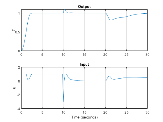
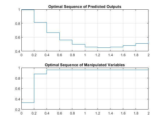
To check the optimal predicted trajectories at any point during the simulation, you can use the second output argument of mpcmove. For this example, assume you start from the current state (x and xmpc). Also assume that, from this point until the end of the horizon, the reference set-point is 0.5 and the disturbance is 0. Simulate the controller and return the info structure.

r = 0.5;                                    % reference
v = 0;                                      % disturbance
[~,info] = mpcmove(mpcobj,xmpc,y,r,v);      % solve over prediction horizon

Display the info variable.

info

info = 

  struct with fields:

          Uopt: [11x1 double]
          Yopt: [11x1 double]
          Xopt: [11x6 double]
          Topt: [11x1 double]
         Slack: 0
    Iterations: 1
        QPCode: 'feasible'
          Cost: 0.1399

info is a structure containing the predicted optimal sequences of manipulated variables, plant states, and outputs over the prediction horizon. mpcmove calculated this sequence, together with the optimal first move, by solving a quadratic optimization problem to minimize the cost function. The plant states and outputs in info result from applying the optimal manipulated variable sequence directly to mpcobj.Model.Plant, in an open-loop fashion. Due to the presence of noise, unmeasured disturbances, and uncertainties, this open-loop optimization process is not equivalent to simulating the closed loop consisting of the plant, estimator and controller using either the sim command or mpcmove iteratively in a for loop.

Extract the predicted optimal trajectories.

topt = info.Topt;                    % time
yopt = info.Yopt;                    % predicted optimal plant model outputs
uopt = info.Uopt;                    % predicted optimal mv sequence

Since the optimal sequence values are constant across each control step, plot the trajectories using a stairstep plot.

figure                                              % create new figure

subplot(2,1,1)                                      % create upper subplot
stairs(topt,yopt)                                   % plot yopt in a stairstep graph
title('Optimal Sequence of Predicted Outputs')      % add title to upper subplot
grid                                                % add grid to upper subplot

subplot(2,1,2)                                      % create lower subplot
stairs(topt,uopt)                                   % plot uopt in a stairstep graph
title('Optimal Sequence of Manipulated Variables')  % add title to upper subplot
grid                                                % add grid to upper subplot

Linear Representation of MPC Controller

When the constraints are not active, the MPC controller behaves like a linear controller. Note that for a finite-time unconstrained Linear Quadratic Regulator problem with a finite non-receding horizon, the value function is time-dependent, which causes the optimal feedback gain to be time varying. In contrast, in MPC the horizon has a constant length because it is always receding, resulting in a time-invariant value function and consequently a time-invariant optimal feedback gain.

You can get the state-space form of the MPC controller.

LTI = ss(mpcobj,'rv');                  % get state-space representation

Get the state-space matrices to simulate the linearized controller.

[AL,BL,CL,DL] = ssdata(LTI);            % get state-space matrices

Initialize variables for a closed-loop simulation of both the original MPC controller without constraints and the linearized controller.

mpcobj.MV = [];             % remove input constraints
mpcobj.OV = [];             % remove output constraints

Tstop = 5;                  % set simulation time
y = 0;                      % set initial measured output
r = 1;                      % set output reference set-point (constant)
u = 0;                      % set previous (initial) input command

x = [0 0 0 0 0]';           % set initial state of plant
xmpc = mpcstate(mpcobj);    % set initial state of unconstrained MPC controller
xL = zeros(size(BL,1),1);   % set initial state of linearized MPC controller

YY = [];                    % define workspace array to store plant outputs

   Assuming no disturbance added to measured output #1.
-->"Model.Noise" is empty. Assuming white noise on each measured output.

Simulate both controllers in a closed loop with the same plant model.

for k = 0:round(Tstop/Ts)-1

    YY = [YY,y];            % store current output for plotting purposes

    % Define measured disturbance signal v(k).
    v = 0;
    if k*Ts>=10
        v = 1;              % raising to 1 after 10 seconds
    end

    % Define unmeasured disturbance signal d(k).
    d = 0;
    if k*Ts>=20
        d = -0.5;           % falling to -0.5 after 20 seconds
    end

    % Compute the control actions of both (unconstrained) MPC and linearized MPC
    uMPC = mpcmove(mpcobj,xmpc,y,r,v);   % unconstrained MPC (also updates xmpc)
    u = CL*xL + DL*[y;r;v];              % unconstrained linearized MPC

    % Compare the two control actions
    dispStr(k+1) = {sprintf(['t=%5.2f, u=%7.4f (provided by LTI), u=%7.4f' ...
        ' (provided by MPCOBJ)'],k*Ts,u,uMPC)}; %#ok<*SAGROW>

    % Update state of unconstrained linearized MPC controller
    xL = AL*xL + BL*[y;r;v];

    % Update plant state
    x = A*x + B(:,1)*u + B(:,2)*v + B(:,3)*d;

    % Calculate plant output
    y = C*x + D(:,1)*u + D(:,2)*v + D(:,3)*d;       % D(:,1)=0

end

Display the character arrays containing the control actions.

for k=0:round(Tstop/Ts)-1
    disp(dispStr{k+1});             % display each string as k increases
end

t= 0.00, u= 5.2478 (provided by LTI), u= 5.2478 (provided by MPCOBJ)
t= 0.20, u= 3.0134 (provided by LTI), u= 3.0134 (provided by MPCOBJ)
t= 0.40, u= 0.2281 (provided by LTI), u= 0.2281 (provided by MPCOBJ)
t= 0.60, u=-0.9952 (provided by LTI), u=-0.9952 (provided by MPCOBJ)
t= 0.80, u=-0.8749 (provided by LTI), u=-0.8749 (provided by MPCOBJ)
t= 1.00, u=-0.2022 (provided by LTI), u=-0.2022 (provided by MPCOBJ)
t= 1.20, u= 0.4459 (provided by LTI), u= 0.4459 (provided by MPCOBJ)
t= 1.40, u= 0.8489 (provided by LTI), u= 0.8489 (provided by MPCOBJ)
t= 1.60, u= 1.0192 (provided by LTI), u= 1.0192 (provided by MPCOBJ)
t= 1.80, u= 1.0511 (provided by LTI), u= 1.0511 (provided by MPCOBJ)
t= 2.00, u= 1.0304 (provided by LTI), u= 1.0304 (provided by MPCOBJ)
t= 2.20, u= 1.0053 (provided by LTI), u= 1.0053 (provided by MPCOBJ)
t= 2.40, u= 0.9920 (provided by LTI), u= 0.9920 (provided by MPCOBJ)
t= 2.60, u= 0.9896 (provided by LTI), u= 0.9896 (provided by MPCOBJ)
t= 2.80, u= 0.9925 (provided by LTI), u= 0.9925 (provided by MPCOBJ)
t= 3.00, u= 0.9964 (provided by LTI), u= 0.9964 (provided by MPCOBJ)
t= 3.20, u= 0.9990 (provided by LTI), u= 0.9990 (provided by MPCOBJ)
t= 3.40, u= 1.0002 (provided by LTI), u= 1.0002 (provided by MPCOBJ)
t= 3.60, u= 1.0004 (provided by LTI), u= 1.0004 (provided by MPCOBJ)
t= 3.80, u= 1.0003 (provided by LTI), u= 1.0003 (provided by MPCOBJ)
t= 4.00, u= 1.0001 (provided by LTI), u= 1.0001 (provided by MPCOBJ)
t= 4.20, u= 1.0000 (provided by LTI), u= 1.0000 (provided by MPCOBJ)
t= 4.40, u= 0.9999 (provided by LTI), u= 0.9999 (provided by MPCOBJ)
t= 4.60, u= 1.0000 (provided by LTI), u= 1.0000 (provided by MPCOBJ)
t= 4.80, u= 1.0000 (provided by LTI), u= 1.0000 (provided by MPCOBJ)

Plot the results.

figure                                              % create figure
plot(0:Ts:Tstop-Ts,YY)                              % plot plant outputs
grid                                                % add grid
title('Unconstrained MPC control: Plant output')    % add title
xlabel('Time (seconds)')                            % add label to x axis
ylabel('y')                                         % add label to y axis

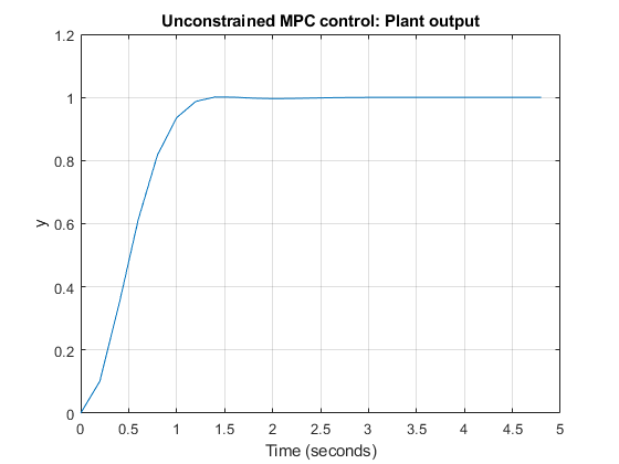
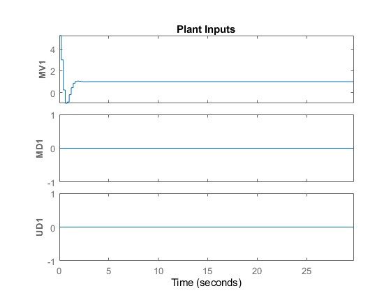
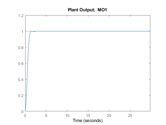
Running a closed-loop simulation in which all controller constraints are turned off is easier using sim, as you just need to specify 'off' in the Constraint field of the related mpcsimopt simulation option object.

SimOptions = mpcsimopt;                     % create simulation options object
SimOptions.Constraints = 'off';             % remove all MPC constraints
SimOptions.UnmeasuredDisturbance = d;       % unmeasured input disturbance
sim(mpcobj,Nf,r,v,SimOptions);              % run closed-loop simulation

Simulate Using Simulink

You can also simulate your MPC controller in Simulink.

To compare results, recreate the MPC object with the constraints you use in the Design MPC Controller section, and the default estimator.

mpcobj = mpc(plantDSS,Ts,10,3);
mpcobj.MV = struct('Min',0,'Max',1,'RateMin',-10,'RateMax',10);
mpcobj.Model.Disturbance = tf(sqrt(1000),[1 0]);

-->"Weights.ManipulatedVariables" is empty. Assuming default 0.00000.
-->"Weights.ManipulatedVariablesRate" is empty. Assuming default 0.10000.
-->"Weights.OutputVariables" is empty. Assuming default 1.00000.

Obtain the state-space matrices of the continuous-time plant.

[A,B,C,D] = ssdata(plantCSS);       % get state-space realization

Open the mpc_miso Simulink model for closed-loop simulation. The plant model is implemented with a continuous state-space block.

open_system('mpc_miso')

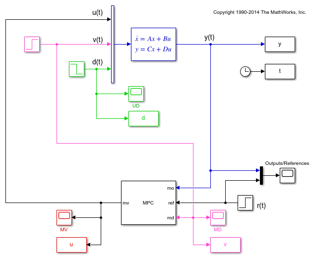
The plant input signals u(t), v(t), and d(t) represent the manipulated variable, measured input disturbance, and unmeasured input disturbance, respectively, while y(t) is the measured output. The block parameters are the matrices forming the state-space realization of the continuous-time plant, and the initial conditions for the five states. The MPC controller is implemented with an MPC Controller block, which has the workspace MPC object mpcobj as a parameter, the manipulated variable as the output, and the measured plant output, reference signal, and measured plant input disturbance, respectively, as inputs. The four Scope blocks plot the five loop signals, which are also saved (except for the reference signal) by four To-Workspace blocks.

Simulate the closed loop system using the Simulink sim command. Note that this command (which simulates a Simulink model, and is equivalent to clicking the "Run" button in the model) is different from the sim command provided by the MPC toolbox (which instead simulates an MPC controller in a loop with an LTI plant).

sim('mpc_miso')

   Assuming no disturbance added to measured output #1.
-->"Model.Noise" is empty. Assuming white noise on each measured output.

To show the simulation results, open the four Scope windows

open_system('mpc_miso/MV')
open_system('mpc_miso/Outputs//References')
open_system('mpc_miso/MD')
open_system('mpc_miso/UD')

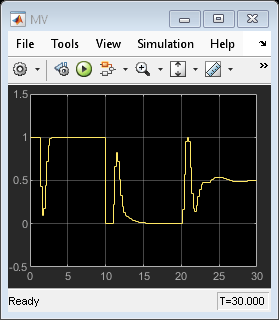
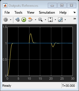
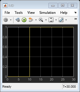
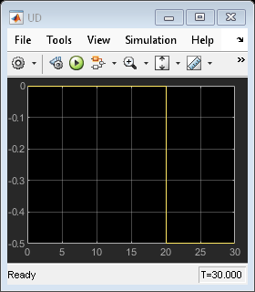
The plots in the Scope windows are equivalent to the ones in the Simulate Closed-Loop Response Using the sim Command and Simulate Closed-Loop Response with Model Mismatch sections, with minor differences due to the fact that in Simulate Closed-Loop Response Using the sim Command the unmeasured disturbance signal is zero, and that in Simulate Closed-Loop Response with Model Mismatch you add noise to the plant input and output. Also note that, while the MPC sim command internally discretizes any continuous plant model using the ZOH method, Simulink typically uses an integration algorithm (in this example ode45) to simulate the closed loop when a continuous-time block is present.

Run Simulation with Sinusoidal Output Noise

Assume output measurements are affected by a sinusoidal disturbance (a single tone sensor noise) of frequency 0.1 Hz.

omega = 2*pi/10;                            % disturbance radial frequency

Open the mpc_misonoise Simulink model, which is similar to the mpc_miso model except for the sinusoidal disturbance added to the measured output. Also, the simulation time is longer and the unmeasured disturbance begins before the measured disturbance.

open_system('mpc_misonoise')                % open new Simulink model

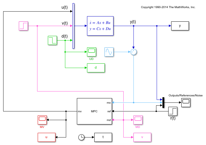
Since this noise is expected, you can specify a noise model to help the state estimator ignore it. Doing so improves the disturbance rejection capabilities of the controller.

mpcobj.Model.Noise = 0.5*tf(omega^2,[1 0 omega^2]); % measurement noise model

Revise the MPC design by specifying a disturbance model on the unmeasured input as a white Gaussian noise with zero mean and variance 0.1.

setindist(mpcobj,tf(0.1));                          % static gain

In this case, you cannot have integrators as disturbance model on both the unmeasured input and the output, because this violates state observability. Therefore when you specify a static gain for the input disturbance model, an output disturbance model consisting in a discretized integrator is automatically added to the controller. This output disturbance model helps the controller to reject step-like and slowly varying disturbances at the output.

getoutdist(mpcobj)

-->Assuming output disturbance added to measured output #1 is integrated white noise.
-->A feedthrough channel in NoiseModel was inserted to prevent problems with estimator design.

ans =
 
  A = 
       x1
   x1   1
 
  B = 
        u1
   x1  0.2
 
  C = 
        x1
   MO1   1
 
  D = 
        u1
   MO1   0
 
Sample time: 0.2 seconds
Discrete-time state-space model.

Large measurement noise can decrease the accuracy of the state estimates. To make the controller less aggressive, and decrease its noise sensitivity, decrease the weight on the output variable tracking.

mpcobj.weights = struct('MV',0,'MVRate',0.1,'OV',0.005);    % new weights

To give the Kalman filter more time to successfully estimate the states, increase the prediction horizon to 40.

mpcobj.predictionhorizon = 40;                  % new prediction horizon

Run the simulation for 145 seconds.

sim('mpc_misonoise',145)	% the second argument is the simulation duration

-->Assuming output disturbance added to measured output #1 is integrated white noise.
-->A feedthrough channel in NoiseModel was inserted to prevent problems with estimator design.

To show the simulation results, open the four Scope windows

open_system('mpc_misonoise/MV')
open_system('mpc_misonoise/Outputs//References//Noise')
open_system('mpc_misonoise/MD')
open_system('mpc_misonoise/UD')

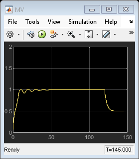
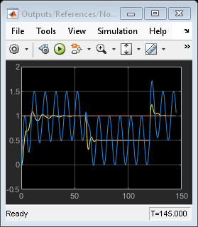
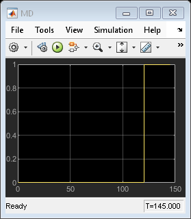
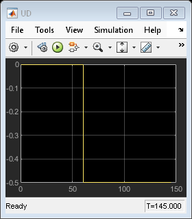
The Kalman filter successfully learns to ignore the measurement noise after 50 seconds. The unmeasured and measured disturbances get rejected in a 10 to 20 second timespan. As expected, the manipulated variable stays in the interval between 0 and 1.

bdclose all    % close all open Simulink models without saving any change
close all      % close all open figures