Control Quarter-Car Suspension Dynamics Using ADMM Solver
This example shows how to design a model predictive controller (MPC) for a quarter-car suspension system, employing the alternating direction method of multipliers (ADMM) solver to control the dynamics of active suspension. The MPC controller leverages a predictive model to anticipate and mitigate the impact of road irregularities and load shifts, ensuring optimal vehicle stability and passenger comfort.
Quarter-Car Suspension Model
The quarter-car suspension model is a two degrees of freedom system that simplifies the vehicle suspension system by focusing on the vertical dynamics of one wheel and a quarter of the car body mass. This model comprises two masses: the sprung mass , which corresponds to the vehicle body, and the unsprung mass , which represents the wheel assembly. The spring and damper of the suspension, with constants and respectively, link the two masses, while the tire is modeled as a spring with constant . Active suspension forces are introduced through the control input , and the road effect is modeled by the excitation . The equations governing the system dynamics are:
, where.
Define the state vector as:
, where and .
The quarter-car suspension model is implemented using a linear state-space system.
% Physical parameters
ms = 300;    % kg
mu = 60;     % kg
bs = 1000;   % N/m/s
ks = 16000;  % N/m
kt = 190000; % N/m

% Define the mass matrix M.
M = [ms 0; 0 mu];
% Define the stiffness matrix F.
F = [-ks ks; ks -(ks + kt)];
% Define the damping matrix B.
B = [-bs bs; bs -bs];
% Define the input matrix q.
q = [1; -1];
% Define the disturbance matrix d.
d = [0; kt];

% Define the state space matrices.
A = [zeros(2,2), eye(2,2); M\F, M\B];
B = [zeros(2,2); M\q M\d];
C = [1 -1 0 0];
D = 0;
plant = ss(A,B,C,D);
Road Disturbance Profile
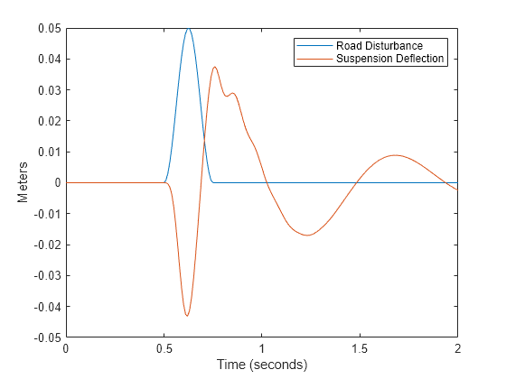
For this example, the road disturbance is modeled as a sinusoidal bump with a frequency of Hz. The disturbance is active only between and seconds to simulate a single bump encounter by the vehicle. The amplitude of the disturbance is scaled by a factor (for this example, 0.025) to represent the severity of the bump.
% Define the frequency of the road disturbance.
f = 4; % Hz
Tstop = 2;

% Define the sampling time.
Ts = 0.01;

% Create a time vector from 0 to Tstop.
% with increments of Ts.
T = (0:Ts:Tstop)';

% Define the road disturbance profile.
v = 0.025*(1 - cos(2*pi*f*T));

% Activate the disturbance only between 2/f and 3/f seconds.
v(T < 2*1/f) = 0;
v(T > 3*1/f) = 0;
Represent the road disturbance profile as a column vector [0 v] for simulation.
Unn = zeros(length(T),2);
Unn(:,2) = v;
Simulate the suspension system without the active control input to provide a baseline response of the system when subjected to the defined road disturbance.
% Use lsim to simulate the uncontrolled system response.
[Yuc,Tuc,Xuc] = lsim(plant,Unn,T);
Plot the impact of the road disturbance on the quarter-car suspension system along with the suspension deflection over time.
figure
title("Response of Uncontrolled Suspension to Road Disturbance")
plot(T, v, "DisplayName", "Road Disturbance");
hold on
plot(Tuc, Yuc, "DisplayName", "Suspension Deflection");
hold off
legend
ylabel("Meters")
xlabel("Time (seconds)")
Design Model Predictive Controller
By default, all input signals of the plant state-space model are manipulated variables, and all outputs are measured outputs. Define the second input signal of the model as a measured disturbance that corresponds to the road effect.
plant = setmpcsignals(plant,"MD",2);-->Assuming unspecified input signals are manipulated variables.
Create an MPC controller for a prediction horizon of 40 steps, a control horizon of 4 steps, and a sampling time of 0.01 second.
Ts = 1e-2;
p = 40;
m = 4;
mpcobj = mpc(plant,Ts,p,m);
-->"Weights.ManipulatedVariables" is empty. Assuming default 0.00000.
-->"Weights.ManipulatedVariablesRate" is empty. Assuming default 0.10000.
-->"Weights.OutputVariables" is empty. Assuming default 1.00000.
Constrain the output variable to the range [-0.05, 0.05].
mpcobj.OutputVariables(1).Min = -0.05;
mpcobj.OutputVariables(1).Max = 0.05;
Set MPC controller parameters to define the scale factor and weights. The scale factor normalizes the output variables, and the weights specify the relative importance of each variable in the cost function. In this case, more emphasis (that is, more cost) is placed on the control input variations by setting a higher weight for the rate of the manipulated variables.
mpcobj.OutputVariables(1).ScaleFactor = 1e-5; mpcobj.Weights.ManipulatedVariables =1; mpcobj.Weights.ManipulatedVariablesRate =
10; mpcobj.Weights.OutputVariables =
5;
Review the MPC controller design to ensure it is configured as intended. The review function generates a design review of the MPC controller.
review(mpcobj)
-->Converting model to discrete time.
-->Integrator added as output disturbance model for measured output #1.
-->"Model.Noise" is empty. Assuming white noise on each measured output.
Test report has been saved to:
 /tmp/Bdoc26a_3233028_1818393/index.html

Define the reference signal r as a vector of zeros, which represents the desired output of no suspension deflection. Define the road disturbance v for the simulation, scaled to represent the severity of the bump and active only within the window of 2/f to 3/f seconds. Then set the simulation options for the MPC controller, specifying that the controller does not anticipate future measured disturbances.
% Define the reference signal as a vector of zeros.
r = zeros(length(T),1);

% Define the road disturbance "v" for the simulation.
v = 0.025 * (1 - cos(2*pi*f*T));
v(T < 2*1/f) = 0;
v(T > 3*1/f) = 0;

% Set simulation options for the MPC controller.
params = mpcsimopt;
params.MDLookAhead = "off";
Set the Optimization Solver
The 'active-set' algorithm is the default optimization method for MPC problems that contain only continuous manipulated variables. The Optimizer property of an mpc object typically has this type of structure.
mpcobj.Optimizer
ans = struct with fields:
         OptimizationType: 'QP'
                   Solver: 'active-set'
            SolverOptions: [1×1 mpc.solver.options.qp.ActiveSet]
             MinOutputECR: 0
    UseSuboptimalSolution: 0
             CustomSolver: 0
      CustomSolverCodeGen: 0
Because the manipulated variable is continuous, the optimization problem is a quadratic programming (QP) one. If you have finite (discrete) control sets, the problem becomes a mixed-Integer Quadratic Programming (MIQP) problem. For more information, see Finite Control Set MPC.
For this example, specify the ADMM solver, which is well-suited for large-scale and distributed optimization problems.
mpcobj.Optimizer.Solver = "admm";To modify the solver parameters and tailor the optimization process to specific requirements, you can access and adjust the settings through the SolverOptions property of the Optimizer property within the MPC object. The SolverOptions property allows you to fine-tune several aspects of the solver behavior, such as convergence tolerances and iteration limit options.
mpcobj.Optimizer.SolverOptions
ans =
  ADMM with properties:

               AbsoluteTolerance: 1.0000e-03
               RelativeTolerance: 1.0000e-03
                   MaxIterations: 1000
             RelaxationParameter: 1.6000
                PenaltyParameter: 0.1000
                        StepSize: 1.0000e-06
    PrimalInfeasibilityTolerance: 1.0000e-04
      DualInfeasibilityTolerance: 1.0000e-04
                    EnablePolish: 0
            PolishRegularization: 1.0000e-06
                 PolishTolerance: 1.0000e-08
             PolishMaxIterations: 3
Simulate the closed-loop system using the 'admm' solver.
[Yad, Tad, Uad, XPad, XCad] = sim(mpcobj,Tstop/Ts + 1,r,v,params);
-->Converting model to discrete time.
-->Integrator added as output disturbance model for measured output #1.
-->"Model.Noise" is empty. Assuming white noise on each measured output.
Then simulate the system using the 'active-set' solver. This algorithm is the default options available for solving the QP problem at each control interval.
mpcobj.Optimizer.Solver = "active-set";
[Yas, Tas, Uas, XPas, XCas] = sim(mpcobj,Tstop/Ts + 1,r,v,params);
-->Converting model to discrete time. -->Integrator added as output disturbance model for measured output #1. -->"Model.Noise" is empty. Assuming white noise on each measured output.
Finally, simulate the system using the 'interior-point' solver. This algorithm is another option for solving the QP problem and might offer different performance characteristics compared to the 'active-set' algorithm.
mpcobj.Optimizer.Solver = "interior-point";
[Yip, Tip, Uip, XPip, XCip] = sim(mpcobj,Tstop/Ts + 1,r,v,params);
-->Converting model to discrete time. -->Integrator added as output disturbance model for measured output #1. -->"Model.Noise" is empty. Assuming white noise on each measured output.
Plot the results of the three simulations. For the code of the plotResults helper function, see Helper Function.
TT = {Tas, Tip, Tad, Tuc};
XX = {Yas, Yip, Yad, Yuc};
UU = {Uas, Uip, Uad, Tuc*0};

plotResults(TT,XX,UU)
subplot(211);
legend("active-set","interior-point","admm","uncontrolled")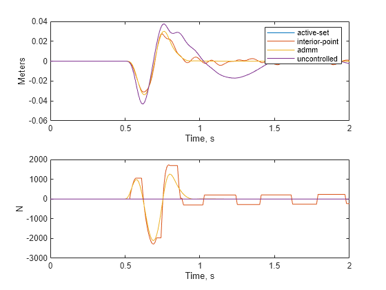
Close the review window.
mlreportgen.utils.rptviewer.close(fullfile(tempdir,'index.html'));Helper Function
This code defines the plotResults helper function. The function plots the results of the simulations to compare their performance. The plots show the system output (suspension deflection) and control input (active suspension force) over time.
function plotResults(TT,XX,UU)

subplot(211);
for i = 1:length(TT)
    plot(TT{i}, XX{i})
    hold on;
end
ylabel("Meters")
xlabel("Time, s")

subplot(212);
for i = 1:length(TT)
    plot(TT{i}, UU{i})
    hold on;
end
ylabel("N")
xlabel("Time, s")
end