Simulate and Generate Code for MPC Controller with Custom QP Solver
This example shows how to simulate and generate code for a model predictive controller that uses a custom quadratic programming (QP) solver. The plant for this example is a dc-servo motor in Simulink®.
DC-Servo Motor Model
The dc-servo motor model is a linear dynamic system described in [1]. plant is the continuous-time state-space model of the motor. tau is the maximum admissible torque, which you use as an output constraint.
[plant,tau] = mpcmotormodel;
Design MPC Controller
The plant has one input, the motor input voltage. The MPC controller uses this input as a manipulated variable (MV). The plant has two outputs, the motor angular position and shaft torque. The angular position is a measured output (MO), and the shaft torque is unmeasured (UO).
plant = setmpcsignals(plant,'MV',1,'MO',1,'UO',2);
Constrain the manipulated variable to be between +/- 220 volts. Since the plant inputs and outputs are of different orders of magnitude, to facilitate tuning, use scale factors. Typical choices of scale factor are the upper/lower limit or the operating range.
MV = struct('Min',-220,'Max',220,'ScaleFactor',440);
There is no constraint on the angular position. Specify upper and lower bounds on shaft torque during the first three prediction horizon steps. To define these bounds, use tau.
OV = struct('Min',{-Inf, [-tau;-tau;-tau;-Inf]}, ...
    'Max',{Inf, [tau;tau;tau;Inf]},'ScaleFactor',{2*pi, 2*tau});
The control task is to achieve zero tracking error for the angular position. Because you only have one manipulated variable, allow shaft torque to float within its constraint by setting its tuning weight to zero.
Weights = struct('MV',0,'MVRate',0.1,'OV',[0.1 0]);
Specify the sample time and horizons, and create the MPC controller, using plant as the predictive model.
Ts = 0.1;           % Sample time
p = 10;             % Prediction horizon
m = 2;              % Control horizon
mpcobj = mpc(plant,Ts,p,m,Weights,MV,OV);
Simulate in Simulink with Built-In QP Solver
To run the remaining example, Simulink is required.
if ~mpcchecktoolboxinstalled('simulink')
    disp('Simulink is required to run this example.')
    return
end
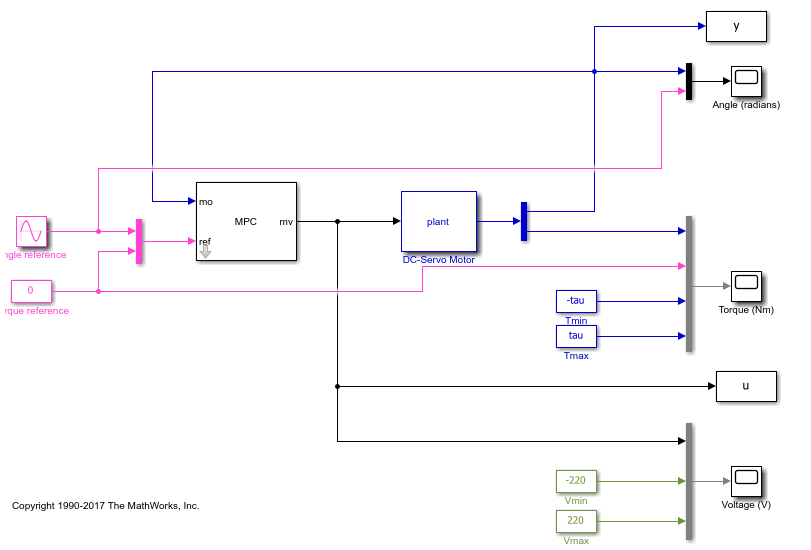
Open a Simulink model that simulates closed-loop control of the dc-servo motor using the MPC controller. By default, MPC uses a built-in QP solver that uses the KWIK algorithm.
mdl = 'mpc_customQPcodegen';
open_system(mdl)
Run the simulation
sim(mdl)
-->Converting model to discrete time.
   Assuming no disturbance added to measured output #1.
-->"Model.Noise" is empty. Assuming white noise on each measured output.
Store the plant input and output signals in the MATLAB workspace.
uKWIK = u;
yKWIK = y;
Simulate in Simulink with a Custom QP Solver
To examine how the custom solver behaves under the same conditions, enable the custom solver in the MPC controller.
mpcobj.Optimizer.CustomSolver = true;
You must also provide a MATLAB® function that satisfies the following requirements:
Function name must be
mpcCustomSolver.Input and output arguments must match the arguments in the template file.
Function must be on the MATLAB path.
In this example, use the custom QP solver defined in the template file mpcCustomSolverCodeGen_TemplateEML.txt, which implements the dantzig algorithm and is suitable for code generation. Save the function in your working folder as mpcCustomSolver.m.
src = which('mpcCustomSolverCodeGen_TemplateEML.txt');
dest = fullfile(pwd,'mpcCustomSolver.m');
copyfile(src,dest,'f')
Simulate closed-loop control of the dc-servo motor, and save the plant input and output.
sim(mdl)
uDantzigSim = u;
yDantzigSim = y;
-->Converting model to discrete time.
   Assuming no disturbance added to measured output #1.
-->"Model.Noise" is empty. Assuming white noise on each measured output.
Generate Code with Custom QP Solver
To run the remaining example, Simulink Coder product is required.
if ~mpcchecktoolboxinstalled('simulinkcoder')
    disp('Simulink(R) Coder(TM) is required to run this example.')
    return
end
To generate code from an MPC Controller block that uses a custom QP solver, enable the custom solver for code generation option in the MPC controller.
mpcobj.Optimizer.CustomSolverCodeGen = true;
You must also provide a MATLAB® function that satisfies all the following requirements:
Function name must be
mpcCustomSolverCodeGen.Input and output arguments must match the arguments in the template file.
Function must be on the MATLAB path.
In this example, use the same custom solver defined in mpcCustomSolverCodeGen_TemplateEML.txt. Save the function in your working folder as mpcCustomSolverCodeGen.m.
src = which('mpcCustomSolverCodeGen_TemplateEML.txt');
dest = fullfile(pwd,'mpcCustomSolverCodeGen.m');
copyfile(src,dest,'f')
Review the saved mpcCustomSolverCodeGen.m file.
function [x, status] = mpcCustomSolverCodeGen(H, f, A, b, x0)
%#codegen
% mpcCustomSolverCodeGen allows the user to specify a custom (QP) solver
% written in MATLAB to be used by MPC controller in code generation.
%
% Workflow:
%   (1) Copy this template file to your work folder and rename it to
%       "mpcCustomSolverCodeGen.m".  The work folder must be on the path.
%   (2) Modify the "mpcCustomSolverCodeGen.m" to use your solver.
%       Note that your solver must use only fixed-size data.
%   (3) Set "mpcobj.Optimizer.CustomSolverCodeGen = true" to tell the MPC
%       controller to use the solver in code generation.
% To generate code:
%   In MATLAB, use "codegen" command with "mpcmoveCodeGeneration" (require MATLAB Coder)
%   In Simulink, generate code with MPC and Adaptive MPC blocks
%
% To use this solver for simulation in MATLAB and Simulink, you need to:
%   (1) Copy "mpcCustomSolver.txt" template file to your work folder and
%       rename it to "mpcCustomSolver.m".  The work folder must be on the path.
%   (2) Modify the "mpcCustomSolver.m" to use your solver.
%   (3) Set "mpcobj.Optimizer.CustomSolver = true" to tell the MPC
%       controller to use the solver in simulation.
%
% The MPC QP problem is defined as follows:
%
%       min J(x) = 0.5*x'*H*x + f'*x, s.t. A*x >= b.
%
% Inputs (provided by MPC controller at run-time):
%       H: a n-by-n Hessian matrix, which is symmetric and positive definite.
%       f: a n-by-1 column vector.
%       A: a m-by-n matrix of inequality constraint coefficients.
%       b: a m-by-1 vector of the right-hand side of inequality constraints.
%      x0: a n-by-1 vector of the initial guess of the optimal solution.
%
% Outputs (sent back to MPC controller at run-time):
%       x: must be a n-by-1 vector of optimal solution.
%  status: must be an integer of:
%           positive value: number of iterations used in computation
%                        0: maximum number of iterations reached
%                       -1: QP is infeasible
%                       -2: Failed to find a solution due to other reasons
% Note that:
%   (1) When solver fails to find an optimal solution (status<=0), "x"
%       still needs to be returned.
%   (2) To use sub-optimal QP solution in MPC, return the sub-optimal "x"
%       with "status = 0".  In addition, you need to set
%       "mpcobj.Optimizer.UseSuboptimalSolution = true" in MPC controller.
%
% DO NOT CHANGE LINES ABOVE

% This template implements a showcase QP solver using "Dantzig" algorithm
% by G. B. Dantzig, A. Orden, and P. Wolfe, "The generalized simplex method
% for minimizing a linear form under linear inequality constraints",
% Pacific J. of Mathematics, 5:183–195, 1955.
%
% User is expected to modify this template and plug in own custom QP solver
% that replaces the "Dantzig" algorithm.

ZERO = zeros('like',H);
ONE = ones('like',H);
% xmin is a constant term that adds to the initial basis because "dantzig"
% requires positive optimization variables.  A fixed "xmin" does not work
% for all MPC problems.
xmin = -1e3*ones(size(f(:)))*ONE;

maxiter = 200*ONE;
nvar = length(f);
ncon = length(b);
a = -H*xmin(:);
H = H\eye(nvar);
rhsc = A*xmin(:) - b(:);
rhsa = a-f(:);
TAB = -[H H*A';A*H A*H*A'];
basisi = [H*rhsa; rhsc + A*H*rhsa];
ibi = -(1:nvar+ncon)'*ONE;
ili = -ibi*ONE;
%% Call EML function "qpdantzg"
[basis,ib,il,iter] = qpdantzg(TAB,basisi,ibi,ili,maxiter); %#ok<ASGLU>
%% status
if iter > maxiter
    status = ZERO;
elseif iter < ZERO
    status = -ONE;
else
    status = iter;
end
%% optimal variable
x = zeros(nvar,1,'like',H);
for j = 1:nvar
    if il(j) <= ZERO
        x(j) = xmin(j);
    else
        x(j) = basis(il(j))+xmin(j);
    end
end
Generate executable code from the Simulink model using the slbuild command from Simulink Coder.
slbuild(mdl)
### Searching for referenced models in model 'mpc_customQPcodegen'.
### Total of 1 models to build.
### Starting build procedure for: mpc_customQPcodegen
-->Converting model to discrete time.
   Assuming no disturbance added to measured output #1.
-->"Model.Noise" is empty. Assuming white noise on each measured output.
### Successful completion of build procedure for: mpc_customQPcodegen

Build Summary

Top model targets:

Model                Build Reason                                         Status                        Build Duration
======================================================================================================================
mpc_customQPcodegen  Information cache folder or artifacts were missing.  Code generated and compiled.  0h 0m 21.319s

1 of 1 models built (0 models already up to date)
Build duration: 0h 0m 23.434s
On a Windows system, after the build process finishes, the software adds the executable file mpc_customQPcodegen.exe to your working folder.
Run the executable. After the executable completes successfully (status = 0), the software adds the data file mpc_customQPcodegen.mat to your working folder. Load the data file into the MATLAB workspace, and obtain the plant input and output signals generated by the executable.
if ispc
    status = system(mdl);
    load(mdl)
    uDantzigCodeGen = u;
    yDantzigCodeGen = y;
else
    disp('The example only runs the executable on Windows system.');
end
The example only runs the executable on Windows system.
Compare Simulation Results
Compare the plant input and output signals from all the simulations.
if ispc
    figure
    subplot(2,1,1)
    plot(u.time,uKWIK.signals.values,u.time,uDantzigSim.signals.values, ...
        '+',u.time,uDantzigCodeGen.signals.values,'o')
    subplot(2,1,2)
    plot(y.time,yKWIK.signals.values,y.time,yDantzigSim.signals.values, ...
        '+',y.time,yDantzigCodeGen.signals.values,'o')
    legend('KWIK','Dantzig Simu','Dantzig CodeGen','Location','northwest')
else
    figure
    subplot(2,1,1)
    plot(u.time,uKWIK.signals.values,u.time,uDantzigSim.signals.values,'+')
    subplot(2,1,2)
    plot(y.time,yKWIK.signals.values,y.time,yDantzigSim.signals.values,'+')
    legend('KWIK','Dantzig Simu','Location','northwest')
end
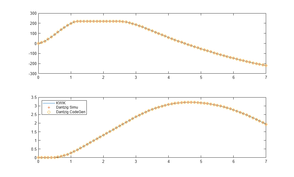
The signals from all the simulations are identical.
References
[1] Bemporad, A. and Mosca, E. "Fulfilling hard constraints in uncertain linear systems by reference managing." Automatica, Vol. 34, Number 4, pp. 451-461, 1998.
bdclose(mdl)

See Also
Objects
Blocks
Topics
- Simulation and Code Generation Using Simulink Coder
- Solve Custom MPC Quadratic Programming Problem and Generate Code
- Implement MPC Controllers Using Embotech FORCESPRO Solvers
- QP Solvers for Linear MPC
- Configure Optimization Solver for Nonlinear MPC
- Generate Code and Deploy Controller to Real-Time Targets