Swing-Up Control of Pendulum Using Nonlinear Model Predictive Control

Pendulum/Cart Assembly

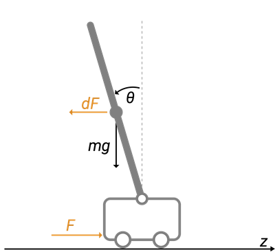
The plant for this example is a pendulum/cart assembly, where z is the cart position and theta is the pendulum angle. The manipulated variable for this system is a variable force F acting on the cart. The range of the force is between -100 and 100. An impulsive disturbance dF can push the pendulum as well.

System Equations

The system is described by the following equations, where l is the distance to the pendulum center of mass, m and M are the masses of the pendulum and the cart, respectively, and Kd is a viscous friction damping term.

From the second equation, you can derive a formula expressing the angular acceleration as a function of the angular and linear velocities by collecting the length l in the second term, the cosine of theta in the last term, and isolating the second derivative of theta on the left hand side. For a thorough explanation of how the equations are derived, see Derive Equations of Motion and Simulate Cart-Pole System (Symbolic Math Toolbox).

The system equations are coded in the file pendulumCT0.m where the impulsive force dF is not included (that is set to zero) because it is considered a disturbance unknown to the controller. Display the file.

type("pendulumCT0.m")

function dxdt = pendulumCT0(x, u)
%% Continuous-time nonlinear dynamic model of a pendulum on a cart
%
% 4 states (x): 
%   cart position (z)
%   cart velocity (z_dot): when positive, cart moves to right
%   angle (theta): when 0, pendulum is at upright position
%   angular velocity (theta_dot): anti-clockwise positive
% 
% 1 inputs: (u)
%   force (F): when positive, force pushes cart to right 
%
% Copyright 2018 The MathWorks, Inc.

%#codegen

%% parameters
M = 1;      % cart mass
m = 1;      % pendulum mass
g = 9.81;   % gravity of earth
l = 0.5;    % pendulum length
Kd = 10;    % cart damping

%% Obtain x, u and y

% x (state variables)
z_dot = x(2);
theta = x(3);
theta_dot = x(4);

% u (input variable)
F = u;

%% Compute dxdt
dxdt = [

    z_dot;...

    (   F - Kd*z_dot ...
        - m*l*theta_dot^2*sin(theta) ...
        + m*g*sin(theta)*cos(theta)  ...
    )/(M + m*sin(theta)^2);...
    
    theta_dot;...

    (  g*sin(theta) + ...
       (F - Kd*z_dot - m*l*theta_dot^2*sin(theta))*cos(theta)/(M + m) ...
    )/(l - m*l*cos(theta)^2/(M + m));
          
   ];

Control Objectives

Assume the following initial conditions for the pendulum/cart assembly.

The control objectives are:

The downward equilibrium position is stable, and the inverted equilibrium position is unstable, which makes swing-up control more challenging for a single linear controller, which nonlinear MPC handles easily.

Control Structure

In this example, the nonlinear MPC controller has the following I/O configuration.

Two other states, cart velocity (zdot) and pendulum angular velocity (thetadot) are not measurable.

While the setpoint of the cart position, z, can vary, the setpoint of the pendulum angle, theta, is always 0 (inverted equilibrium position).

Create Nonlinear MPC Controller

Create a nonlinear MPC controller with the proper dimensions using an nlmpc object. In this example, the prediction model has 4 states, 2 outputs, and 1 input (manipulated variable, or MV).

nx = 4;
ny = 2;
nu = 1;
nlobj = nlmpc(nx, ny, nu);

Zero weights are applied to one or more OVs because there are fewer MVs than OVs.

The prediction model has a sample time of 0.1 seconds, which is the same as the controller sample time.

Ts = 0.1;
nlobj.Ts = Ts;

Set the prediction horizon to 10, which is long enough to capture major dynamics in the plant but not so long that it hurts computational efficiency.

nlobj.PredictionHorizon = 10;

Set the control horizon to 5, which is long enough to give the controller enough degrees of freedom to handle the unstable mode without introducing excessive decision variables.

nlobj.ControlHorizon = 5;

Specify Nonlinear Plant Model

The major benefit of nonlinear model predictive control is that it uses a nonlinear dynamic model to predict plant behavior in the future across a wide range of operating conditions.

This nonlinear model is usually a first principle model consisting of a set of differential and algebraic equations (DAEs). In this example, a discrete-time cart and pendulum system is defined in the pendulumDT0 function. This function integrates the continuous-time model, pendulumCT0, between control intervals using a multistep forward Euler method. The same function is also used by the nonlinear state estimator. Display the discretized model.

type("pendulumDT0.m")

function xk1 = pendulumDT0(xk, uk, Ts)
%% Discrete-time nonlinear dynamic model of a pendulum on a cart at time k
%
% 4 states (xk): 
%   cart position (z)
%   cart velocity (z_dot): when positive, cart moves to right
%   angle (theta): when 0, pendulum is at upright position
%   angular velocity (theta_dot): anticlockwise positive
% 
% 1 inputs: (uk)
%   force (F): when positive, force pushes cart to right 
%
% xk1 is the states at time k+1.
%
% Copyright 2018 The MathWorks, Inc.

%#codegen

% Repeat application of Euler method sampled at Ts/Nd.
Nd = 10;
delta = Ts/Nd;
xk1 = xk;
for ct=1:Nd
    xk1 = xk1 + delta*pendulumCT0(xk1,uk);
end
% Note that we choose the Euler method (first order Runge-Kutta method)
% because it is more efficient for plant with non-stiff ODEs.  You can
% choose other ODE solvers such as ode23, ode45 for better accuracy or
% ode15s and ode23s for stiff ODEs.  Those solvers are available from
% MATLAB.

Set the discretized model as the prediction model used by the nonlinear MPC controller.

nlobj.Model.StateFcn = "pendulumDT0";

To use a discrete-time model, set the Model.IsContinuousTime property of the controller to false.

nlobj.Model.IsContinuousTime = false;

The prediction model uses an optional parameter, Ts, to represent the sample time. Using this parameter means that, if you change the prediction sample time during the design, you do not have to modify the pendulumDT0 file.

nlobj.Model.NumberOfParameters = 1;

The two plant outputs are the first and third state in the model, the cart position and pendulum angle, respectively. The corresponding output function is defined in the pendulumOutputFcn function.

nlobj.Model.OutputFcn = 'pendulumOutputFcn';

It is best practice to provide analytical Jacobian functions whenever possible, since they significantly improve the simulation speed. In this example, provide a Jacobian for the output function using an anonymous function.

nlobj.Jacobian.OutputFcn = @(x,u,Ts) [1 0 0 0; 0 0 1 0];

Since you do not provide Jacobian for the state function, the nonlinear MPC controller estimates the state function Jacobian during optimization using numerical perturbation. Doing so slows down simulation to some degree.

Define Cost and Constraints

Like linear MPC, nonlinear MPC solves a constrained optimization problem at each control interval. However, since the plant model is nonlinear, nonlinear MPC converts the optimal control problem into a nonlinear optimization problem with a nonlinear cost function and nonlinear constraints.

The cost function used in this example is the same standard cost function used by linear MPC, where output reference tracking and manipulated variable move suppression are enforced. Therefore, specify standard MPC tuning weights.

nlobj.Weights.OutputVariables = [3 3];
nlobj.Weights.ManipulatedVariablesRate = 0.1;

The cart position is limited to the range -10 to 10.

nlobj.OV(1).Min = -10;
nlobj.OV(1).Max = 10;

The force has a range between -100 and 100.

nlobj.MV.Min = -100;
nlobj.MV.Max = 100;

Validate Nonlinear MPC Controller

After designing a nonlinear MPC controller object, it is best practice to check the functions you defined for the prediction model, state function, output function, custom cost, and custom constraints, as well as their Jacobians. To do so, use the validateFcns command. This function detects any dimensional and numerical inconsistencies in these functions.

x0 = [0.1;0.2;-pi/2;0.3];
u0 = 0.4;
validateFcns(nlobj,x0,u0,[],{Ts});

Model.StateFcn is OK.
Model.OutputFcn is OK.
Jacobian.OutputFcn is OK.
Analysis of user-provided model, cost, and constraint functions complete.

State Estimation

In this example, only two plant states (cart position and pendulum angle) are measurable. Therefore, you estimate the four plant states using an extended Kalman filter. Its state transition function is defined in pendulumStateFcn.m and its measurement function is defined in pendulumMeasurementFcn.m.

EKF = extendedKalmanFilter(@pendulumStateFcn, @pendulumMeasurementFcn);

Closed-Loop Simulation in MATLAB

Specify the initial conditions for simulations by setting the initial plant state and output values. Also, specify the initial state of the extended Kalman filter.

The initial conditions of the simulation areas follows.

x = [0;0;-pi;0];
y = [x(1);x(3)];
EKF.State = x;

mv is the optimal control move computed at any control interval. Initialize mv to zero, since the force applied to the cart is zero at the beginning.

mv = 0;

In the first stage of the simulation, the pendulum swings up from a downward equilibrium position to an inverted equilibrium position. The state references for this stage are all zero.

yref1 = [0 0];

At a time of 10 seconds, the cart moves from position 0 to 5. Set the state references for this position.

yref2 = [5 0];

Using the nlmpcmove command, compute optimal control moves at each control interval. This function constructs a nonlinear programming problem and solves it using the fmincon function from the Optimization Toolbox.

Specify the prediction model parameter using an nlmpcmoveopt object, and pass this object to nlmpcmove.

nloptions = nlmpcmoveopt;
nloptions.Parameters = {Ts};

Run the simulation for 20 seconds.

Duration = 20;
hbar = waitbar(0,'Simulation Progress');
xHistory = x;
for ct = 1:(20/Ts)

    % Set references
    if ct*Ts<10
        yref = yref1;
    else
        yref = yref2;
    end

    % Correct previous prediction using current measurement.
    xk = correct(EKF, y);

    % Compute optimal control moves.
    [mv,nloptions,info] = nlmpcmove(nlobj,xk,mv,yref,[],nloptions);

    % Predict prediction model states for the next iteration.
    predict(EKF, [mv; Ts]);

    % Implement first optimal control move and update plant states.
    x = pendulumDT0(x,mv,Ts);

    % Generate sensor data with some white noise.
    y = x([1 3]) + randn(2,1)*0.01;

    % Save plant states for display.
    xHistory = [xHistory x]; %#ok<*AGROW>
    waitbar(ct*Ts/20,hbar);
end
close(hbar)

Plot the closed-loop response.

figure

subplot(2,2,1)
plot(0:Ts:Duration,xHistory(1,:))
xlabel('time')
ylabel('z')
title('cart position')

subplot(2,2,2)
plot(0:Ts:Duration,xHistory(2,:))
xlabel('time')
ylabel('zdot')
title('cart velocity')

subplot(2,2,3)
plot(0:Ts:Duration,xHistory(3,:))
xlabel('time')
ylabel('theta')
title('pendulum angle')

subplot(2,2,4)
plot(0:Ts:Duration,xHistory(4,:))
xlabel('time')
ylabel('thetadot')
title('pendulum velocity')

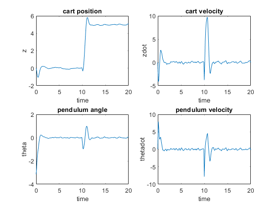
The pendulum angle plot shows that the pendulum successfully swings up in two seconds. During the swing-up process, the cart is displaced with a peak deviation of -1, and returned to its original position around a time of 2 seconds.

The cart position plot shows that the cart successfully moves to z = 5 in two seconds. While the cart moves, the pendulum is displaced with a peak deviation of 1 radian (57 degrees) and returned to an inverted equilibrium position around a time of 12 seconds.

Closed-Loop Simulation with FORCESPRO Solver in MATLAB

You can easily use a third-party nonlinear programming solver together with the nonlinear MPC object designed using Model Predictive Control Toolbox software. For example, if you have FORCESPRO software from Embotech installed, you can use their MPC Toolbox Plugin to generate an efficient custom NLP solver from your nlmpc object and use the solver for simulation and code generation.

First, generate a custom solver using the nlmpcToForces command. You can choose using either an Interior-Point (IP) solver or a Sequential Quadratic Programming (SQP) solver using the nlmpcToForcesOptions command.

options = nlmpcToForcesOptions();
options.SolverName = 'MyIPSolver';
options.SolverType = 'InteriorPoint';
options.Parameter = Ts;
options.x0 = [0;0;-pi;0];
options.mv0 = 0;
[coredata, onlinedata] = nlmpcToForces(nlobj,options);

The nlmpcToForces function generates a custom MEX function nlmpcmove_MyIPSolver, which you can use to speed up closed-loop simulation.

x = [0;0;-pi;0];
mv = 0;
EKF.State = x;
y = [x(1);x(3)];
hbar = waitbar(0,'Simulation Progress');
xHistory = x;
for ct = 1:(20/Ts)

     % Set references
     if ct*Ts<10
         onlinedata.ref = repmat(yref1,10,1);
     else
         onlinedata.ref = repmat(yref2,10,1);
     end

     % Correct previous prediction using current measurement.
     xk = correct(EKF, y);

     % Compute optimal control moves using FORCESPRO solver.
     [mv,onlinedata,info] = nlmpcmove_MyIPSolver(xk,mv,onlinedata);

     % Predict prediction model states for the next iteration.
     predict(EKF, [mv; Ts]);

     % Implement first optimal control move and update plant states.
     x = pendulumDT0(x,mv,Ts);

     % Generate sensor data with some white noise.
     y = x([1 3]) + randn(2,1)*0.01;

     % Save plant states for display.
     xHistory = [xHistory x]; %#ok<*AGROW>
     waitbar(ct*Ts/20,hbar);
 end
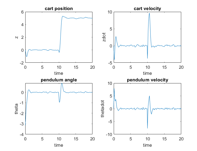
 close(hbar)

As expected, the closed-loop response is similar to the one obtained using fmincon as expected.

Closed-Loop Simulation in Simulink

Validate the nonlinear MPC controller with a closed-loop simulation in Simulink®.

Open the Simulink model.

mdl = 'mpc_pendcartNMPC';
open_system(mdl)

In this model, the Nonlinear MPC Controller block is configured to use the previously designed controller, nlobj.

To use optional parameters in the prediction model, the model has a Simulink Bus block connected to the params input port of the Nonlinear MPC Controller block. To configure this bus block to use the Ts parameter, create a Bus object in the MATLAB® workspace and configure the Bus Creator block to use this object. To do so, use the createParameterBus function. In this example, name the Bus object 'myBusObject'.

createParameterBus(nlobj,[mdl '/Nonlinear MPC Controller'],'myBusObject',{Ts});

Simulink Bus object "myBusObject" created in the MATLAB Workspace.
Bus Creator block "mpc_pendcartNMPC/Nonlinear MPC Controller" is configured to use it.

Run the simulation for 30 seconds.

open_system([mdl '/Scope'])
sim(mdl)

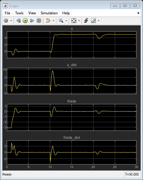
The nonlinear simulation in Simulink produces identical swing-up and cart position tracking results compared to the MATLAB simulation. Also, a push (impulse disturbance dF) is applied to the inverted pendulum at a time of 20 seconds. The nonlinear MPC controller successfully rejects the disturbance and returns the cart to z = 5 and the pendulum to an inverted equilibrium position.

Closed-Loop Simulation with FORCESPRO Solver in Simulink

You can also use the FORCES Nonlinear MPC block from the Embotech FORCESPRO software to simulate the nonlinear MPC using the generated custom NLP solver.

If you have FORCESPRO software installed, simply replace the Nonlinear MPC block in the above model with the FORCESPRO Nonlinear MPC block from the FORCESPRO MPC Blocks section in the library browser. In the block dialog, specify coredata as the controller data structure and enable the model parameter input. Re-connect remaining signals as in the following picture.

The closed-loop response is similar to the one using fmincon.

Conclusion

This example illustrates a general workflow to design and simulate nonlinear MPC in MATLAB and Simulink using an nlmpc object and Nonlinear MPC Controller block, respectively. Depending on the specific nonlinear plant characteristics and control requirements, the implementation details can vary significantly. The key design challenges include:

You can use the functions and Simulink model in this example as templates for other nonlinear MPC design and simulation tasks.

Both the nlmpcmoveCodeGeneration command from Model Predictive Control Toolbox software and the nlmpcmoveForces command from FORCESPRO support code generation in MATLAB. Both the Nonlinear MPC block from Model Predictive Control Toolbox software and FORCES Nonlinear MPC block from FORCESPRO support code generation in Simulink.