Time-Varying MPC Control of a Time-Varying Plant

This example uses:

This example shows how the Model Predictive Control Toolbox™ can use time-varying prediction models to achieve better performance when controlling a time-varying plant.

The following MPC controllers are compared:

Linear MPC controller based on a time-invariant average model
Linear MPC controller based on a time-invariant model, which is updated at each time step
Linear MPC controller based on a time-varying prediction model.

Time-Varying Linear Plant

In this example, the plant is a single-input-single-output 3rd order time-varying linear system with poles, zeros and gain that vary periodically with time.

$G = \frac{{5s + 5 + 2\cos \left( {2.5t} \right)}}{{{s^3}
 + 3{s^2} + 2s + 6 + \sin \left( {5t} \right)}}$

The plant poles move between being stable and unstable at run time, which leads to a challenging control problem.

Generate an array of plant models at t = 0, 0.1, 0.2, ..., 10 seconds.

Models = tf;
ct = 1;
for t = 0:0.1:10
    Models(:,:,ct) = tf([5 5+2*cos(2.5*t)],[1 3 2 6+sin(5*t)]);
    ct = ct + 1;
end

Convert the models to state-space format and discretize them with a sample time of 0.1 second.

Ts = 0.1;
Models = ss(c2d(Models,Ts));

MPC Controller Design

The control objective is to track a step change in the reference signal. First, design an MPC controller for the average plant model. The controller sample time is 0.1 second.

sys = ss(c2d(tf([5 5],[1 3 2 6]),Ts));  % prediction model
p = 3;                                  % prediction horizon
m = 3;                                  % control horizon
mpcobj = mpc(sys,Ts,p,m);

-->"Weights.ManipulatedVariables" is empty. Assuming default 0.00000.
-->"Weights.ManipulatedVariablesRate" is empty. Assuming default 0.10000.
-->"Weights.OutputVariables" is empty. Assuming default 1.00000.

Set hard constraints on the manipulated variable and specify tuning weights.

mpcobj.MV = struct('Min',-2,'Max',2);
mpcobj.Weights = struct('MV',0,'MVRate',0.01,'Output',1);

Set the initial plant states to zero.

x0 = zeros(size(sys.B));

Closed-Loop Simulation with Implicit MPC

Run a closed-loop simulation to examine whether the designed implicit MPC controller can achieve the control objective without updating the plant model used in prediction.

Set the simulation duration to 5 seconds.

Tstop = 5;

Use the mpcmove command in a loop to simulate the closed-loop response.

yyMPC = [];
uuMPC = [];
x = x0;
xmpc = mpcstate(mpcobj);
fprintf('Simulating MPC controller based on average LTI model.\n');
for ct = 1:(Tstop/Ts+1)
    % Get the real plant.
    real_plant = Models(:,:,ct);
    % Update and store the plant output.
    y = real_plant.C*x;
    yyMPC = [yyMPC,y];
    % Compute and store the MPC optimal move.
    u = mpcmove(mpcobj,xmpc,y,1);
    uuMPC = [uuMPC,u];
    % Update the plant state.
    x = real_plant.A*x + real_plant.B*u;
end

-->Assuming output disturbance added to measured output #1 is integrated white noise.
-->"Model.Noise" is empty. Assuming white noise on each measured output.
Simulating MPC controller based on average LTI model.

Closed-Loop Simulation with Adaptive MPC

Run a second simulation to examine whether an adaptive MPC controller can achieve the control objective.

Use the mpcmoveAdaptive command in a loop to simulate the closed-loop response. Update the plant model for each control interval, and use the updated model to compute the optimal control moves. The mpcmoveAdaptive command uses the same prediction model across the prediction horizon.

yyAMPC = [];
uuAMPC = [];
x = x0;
xmpc = mpcstate(mpcobj);
nominal = mpcobj.Model.Nominal;

fprintf(['Simulating MPC controller based on LTI model,' ...
    ' updated at each time step t.\n']);

for ct = 1:(Tstop/Ts+1)
    % Get the real plant.
    real_plant = Models(:,:,ct);
    % Update and store the plant output.
    y = real_plant.C*x;
    yyAMPC = [yyAMPC, y];
    % Compute and store the MPC optimal move.
    u = mpcmoveAdaptive(mpcobj,xmpc,real_plant,nominal,y,1);
    uuAMPC = [uuAMPC,u];
    % Update the plant state.
    x = real_plant.A*x + real_plant.B*u;
end

Simulating MPC controller based on LTI model, updated at each time step t.

Closed-Loop Simulation with Time-Varying MPC

Run a third simulation to examine whether a time-varying MPC controller can achieve the control objective.

The controller updates the prediction model at each control interval and also uses time-varying models across the prediction horizon, which gives MPC controller the best knowledge of plant behavior in the future.

Use the mpcmoveAdaptive command in a loop to simulate the closed-loop response. Specify an array of plant models rather than a single model. The controller uses each model in the array at a different prediction horizon step.

yyLTVMPC = [];
uuLTVMPC = [];
x = x0;
xmpc = mpcstate(mpcobj);
% Nominal conditions are constant over the prediction horizon.
Nominals = repmat(nominal,3,1);

fprintf(['Simulating MPC controller based on time-varying model, ' ...
    'updated at each time step t.\n']);

for ct = 1:(Tstop/Ts+1)
    % Get the real plant.
    real_plant = Models(:,:,ct);
    % Update and store the plant output.
    y = real_plant.C*x;
    yyLTVMPC = [yyLTVMPC, y];
    % Compute and store the MPC optimal move.
    u = mpcmoveAdaptive(mpcobj,xmpc,Models(:,:,ct:ct+p),Nominals,y,1);
    uuLTVMPC = [uuLTVMPC,u];
    % Update the plant state.
    x = real_plant.A*x + real_plant.B*u;
end

Simulating MPC controller based on time-varying model, updated at each time step t.

Performance Comparison of MPC Controllers

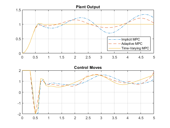
Compare the closed-loop responses.

t = 0:Ts:Tstop;
figure
subplot(2,1,1);
plot(t,yyMPC,'-.',t,yyAMPC,'--',t,yyLTVMPC);
grid
legend('Implicit MPC','Adaptive MPC','Time-Varying MPC', ...
    Location="SouthEast")
title('Plant Output');
subplot(2,1,2)
plot(t,uuMPC,'-.',t,uuAMPC,'--',t,uuLTVMPC)
grid
title('Control Moves');

Only the time-varying MPC controller is able to bring the plant output close enough to the desired setpoint.

Closed-Loop Simulation of Time-Varying MPC in Simulink

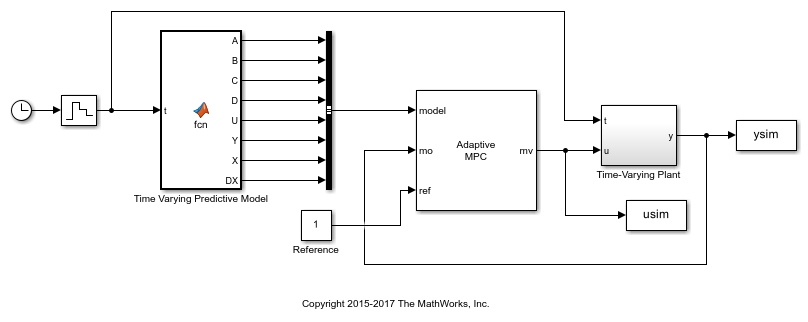
To simulate time-varying MPC control in Simulink®, pass the time-varying plant models to model inport of the Adaptive MPC Controller block.

xmpc = mpcstate(mpcobj);
mdl = 'mpc_timevarying';
open_system(mdl);

Run the simulation.

sim(mdl,Tstop);
fprintf('Simulating MPC controller based on LTV model in Simulink.\n');

Simulating MPC controller based on LTV model in Simulink.

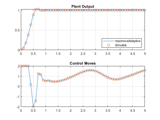
Plot the MATLAB® and Simulink time-varying simulation results.

figure
subplot(2,1,1)
plot(t,yyLTVMPC,t,ysim,'o');
grid
legend('mpcmoveAdaptive','Simulink','Location','SouthEast')
title('Plant Output');
subplot(2,1,2)
plot(t,uuLTVMPC,t,usim,'o')
grid
title('Control Moves');