Truck and Trailer Automatic Parking Using Multistage Nonlinear MPC

Overview

An MPC controller uses an internal model to predict plant behavior. Given the current states of the plant, based on the prediction model, MPC finds an optimal control sequence that minimizes cost and satisfies the constraints specified across the prediction horizon. Because MPC finds the plant future trajectory at the same time, it can work as a powerful tool to solve trajectory optimization problems, such as autonomous parking of a vehicle and motion planning of a robot arm.

In such trajectory optimization problems the plant, cost function, and constraints can often be nonlinear. Therefore, you need to use nonlinear MPC controller for problem formulation and solution. In this example, you design a nonlinear MPC controller that finds an optimal route to automatically park a truck with a single trailer from its initial position to its target position, which is between two static obstacles. You can then pass the generated path to a low-level controller as a reference signal, so that it can execute the parking maneuver in real time.

This example requires Optimization Toolbox™ and Robotics System Toolbox™ software.

Truck and Single Trailer System

The following figure shows the truck and trailer nonlinear dynamic system.

The states for this model are:

The inputs for this model are:

For this model, length and position are in meters, velocity is in m/s, and angles are in radians.

Define the following model parameters.

params = struct('M', 1, ...
    'L1',6,...
    'W1',2.5,...
    'L2',10,...
    'W2',2.5,...
    'Lwheel',1,...
    'Wwheel',0.4);

The nonlinear model is implemented in the TruckTrailerStateFcn function and its manually-derived analytical Jacobian (which is used to speed up optimization) is in the TruckTrailerStateJacobianFcn function.

In this example, since you use MPC as a path planner instead of a low-level path-following controller, the truck's longitudinal velocity is used as one of the manipulated variables instead of the acceleration.

Automatic Parking Problem

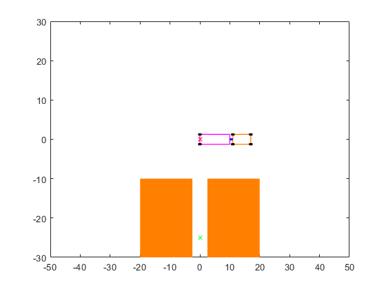
The parking lot is 100 meters wide and 60 meters long. The goal is to find a viable path that brings the truck and trailer system from any initial position to the target position (the green cross in the following figure) in 20 seconds using reverse parking. In the process, the planned path must avoid collisions with two obstacles next to the parking spot.

initialPose = [0;0;0;0];
targetPose = [0;-25;pi/2;0];
TruckTrailerPlot(initialPose,targetPose,params);

The initial plant inputs (steering angle and longitudinal velocity) are both 0.

u0 = zeros(2,1);

The initial position must be valid. Use the inequality constraint function TruckTrailerIneqConFcn to check for validity. Details about this function are discussed in the next section. Here, collision detection is carried out by specific Robotics System Toolbox functions.

cineq = TruckTrailerIneqConFcn(1,initialPose,u0,...
    [params.M;params.L1;params.L2;params.W1;params.W2]);
if any(cineq>0)
    fprintf('Initial pose is not valid.\n');
    return
end

Path Planning Using Multistage Nonlinear MPC

Compared with the generic nonlinear MPC controller (nlmpc object), multistage nonlinear MPC provides you with a more flexible and efficient way to implement MPC with staged costs and constraints. This flexibility and efficiency is especially useful for trajectory planning.

A multistage nonlinear MPC controller with prediction horizon p defines p+1 stages, representing time k (current time), k+1, ..., k+p. For each stage, you can specify stage-specific cost, inequality constraint, and equality constraint functions. These functions depend only on the plant state and input values at that stage. Given the current plant states x[k], MPC finds the manipulated variable (MV) trajectory (from time k to k+p-1) to optimize the summed stage costs (from time k to k+p), satisfying all the stage constraints (from time k to k+p).

In this example, the plant has four states and two inputs (both MVs). Choose the prediction horizon p and sample time Ts such that p*Ts = 20.

Create the multistage nonlinear MPC controller.

p = 40;
nlobj = nlmpcMultistage(p,4,2);
nlobj.Ts = 0.5;

Specify the prediction model and its analytical Jacobian in the controller object. Since the model requires three parameters (M, L1, and L2), set Model.ParameterLength to 3.

nlobj.Model.StateFcn = "TruckTrailerStateFcn";
nlobj.Model.StateJacFcn = "TruckTrailerStateJacobianFcn";
nlobj.Model.ParameterLength = 3;

Specify hard bounds on the two manipulated variables. The steering angle must remain in the range +/- 45 degrees. The maximum forward speed is 10 m/s and the maximum reverse speed is 10 m/s.

nlobj.MV(1).Min = -pi/4;     % Minimum steering angle
nlobj.MV(1).Max =  pi/4;     % Maximum steering angle
nlobj.MV(2).Min = -10;       % Minimum velocity (reverse)
nlobj.MV(2).Max =  10;       % Maximum velocity (forward)

Specify hard bounds on the fourth state, which is the angle between truck and trailer. It cannot go beyond +/-90 degrees due to mechanics limitations.

nlobj.States(4).Min = -pi/2;
nlobj.States(4).Max = pi/2;

You can use different ways to define the cost terms. For example, you might want to minimize time, fuel consumption, or parking speed. For this example, minimize parking speed in the quadratic format to promote safety.

Since MVs are only valid from stage 1 to stage p, you do not need to define any stage cost for the last stage, p+1. The five model settings, M, L1, L2, W1, and W are stage parameters for stages 1 to p and are used by the inequality constraint functions.

for ct=1:p
    nlobj.Stages(ct).CostFcn = "TruckTrailerCost";
    nlobj.Stages(ct).CostJacFcn = "TruckTrailerCostGradientFcn";
    nlobj.Stages(ct).ParameterLength = 5;
end

You can use inequality constraints to avoid collision during the parking process. Use the TruckTrailerIneqConFcn function to check whether the truck or the trailer collide with any of the two static obstacles at a specific stage. When either the truck or the trailer gets within the 1 m safety zone around the obstacles, a collision is detected.

In general, check for such collisions for all the prediction steps (from stage 2 to stage p+1). In this example, however, you only need to check stages from 2 to p because the last stage is already taken care of by the equality constraint function.

For this example, do not provide an analytical Jacobian for the inequality constraint functions because it is too complicated to derive manually. Therefore, the controller uses a finite-difference method (numerical perturbation) to estimate the Jacobian at run time.

for ct=2:p
    nlobj.Stages(ct).IneqConFcn = "TruckTrailerIneqConFcn";
end

Use terminal state for the last stage to ensure successful parking at the target position. In this example, the target position is provided as a run-time signal. Here we use a dummy finite value to let MPC know which states will have terminal values at run time.

nlobj.Model.TerminalState = zeros(4,1);

At the end of multistage nonlinear MPC design, you can use the validateFcns command with random initial plant states and inputs to check whether any of the user-defined state, cost, and constraint function as well as any analytical Jacobian function, has a problem.

You must provide all the defined state functions and stage parameters to the controller at run time. StageParameter contains all the stage parameters stacked into a single vector. We also use TerminalState to specify terminal state at run time.

simdata = getSimulationData(nlobj,'TerminalState');
simdata.StateFcnParameter = [params.M;params.L1;params.L2];
simdata.StageParameter = repmat([params.M;params.L1;params.L2;params.W1;params.W2],p,1);
simdata.TerminalState = targetPose;
validateFcns(nlobj,[2;3;0.5;0.4],[0.1;0.2],simdata);

Model.StateFcn is OK.
Model.StateJacFcn is OK.
"CostFcn" of the following stages [1 2 3 4 5 6 7 8 9 10 11 12 13 14 15 16 17 18 19 20 21 22 23 24 25 26 27 28 29 30 31 32 33 34 35 36 37 38 39 40] are OK.
"CostJacFcn" of the following stages [1 2 3 4 5 6 7 8 9 10 11 12 13 14 15 16 17 18 19 20 21 22 23 24 25 26 27 28 29 30 31 32 33 34 35 36 37 38 39 40] are OK.
"IneqConFcn" of the following stages [2 3 4 5 6 7 8 9 10 11 12 13 14 15 16 17 18 19 20 21 22 23 24 25 26 27 28 29 30 31 32 33 34 35 36 37 38 39 40] are OK.
Analysis of user-provided model, cost, and constraint functions complete.

Since the default nonlinear programming solver fmincon searches for a local minimum, you must provide a good initial guess for the decision variables, especially for trajectory optimization problems that usually involve a complicated (likely nonconvex) solution space.

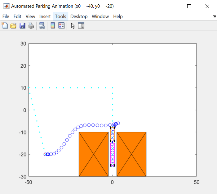
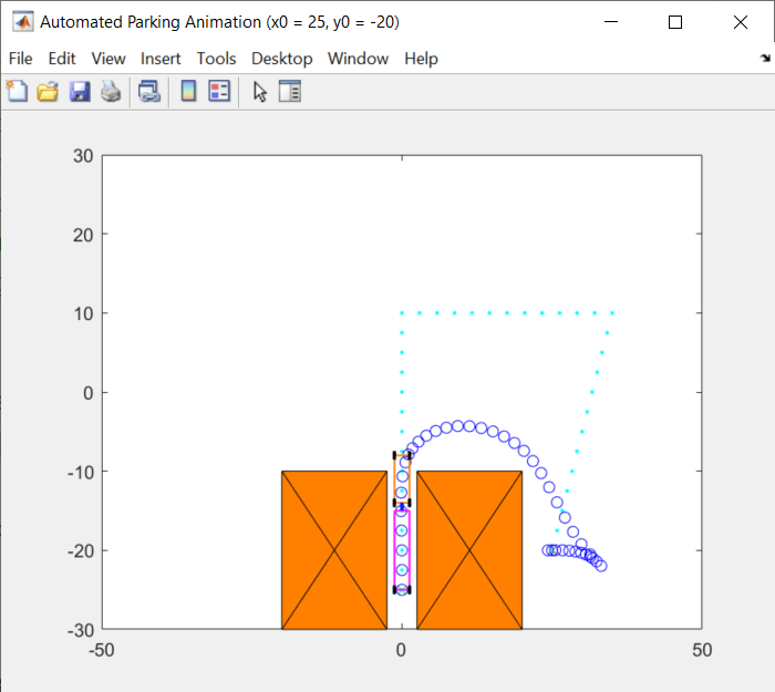
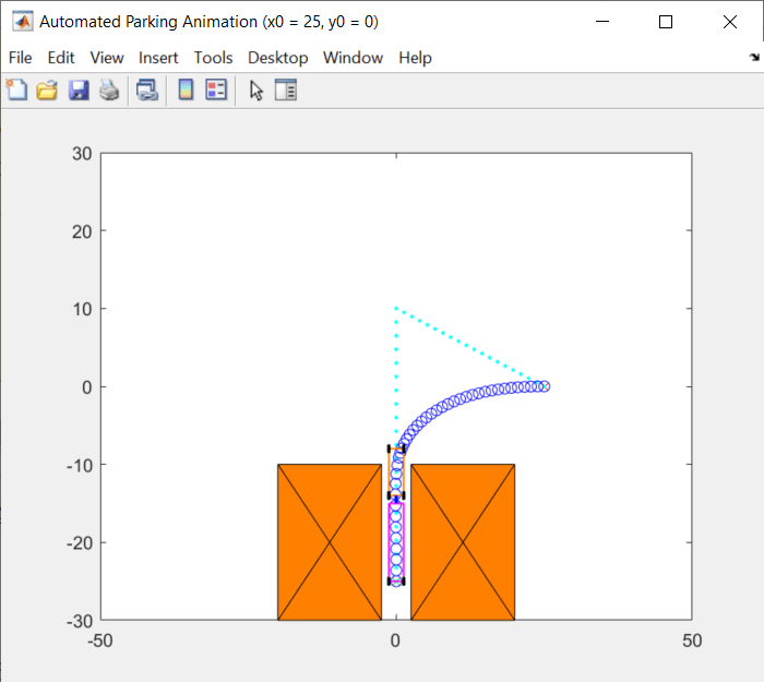
This example has 244 decision variables, the plant states and inputs (6 in total) for each of the first p (40) stages and plant states (4) for the last stage p+1. The TruckTrailerInitialGuess function uses simple heuristics to generate the initial guess. For example, if the truck and trailer is initially positioned above the obstacles, it generates an initial guess with one waypoint; otherwise, it uses two waypoints (a waypoint is an intermediate point on a route of travel at which course is changed). The initial guess is displayed as dots in the following animation plot.

[simdata.InitialGuess, XY0] = TruckTrailerInitialGuess(initialPose,targetPose,u0,p);

Trajectory Planning and Simulation Result

Use the nlmpcmove function to find the optimal parking path, which typically takes ten to twenty seconds, depending on the initial position.

fprintf('Automated Parking Planner is running...\n');
tic;[~,~,info] = nlmpcmove(nlobj,initialPose,u0,simdata);t=toc;
fprintf('Calculation Time = %s; Objective cost = %s; ExitFlag = %s; Iterations = %s\n',...
    num2str(t),num2str(info.Cost),num2str(info.ExitFlag),num2str(info.Iterations));

Automated Parking Planner is running...
Calculation Time = 17.9224; Objective cost = 248.5784; ExitFlag = 1; Iterations = 51

Two plots are generated. One is the animation of the parking process, where blue circles indicate the optimal path and the initial guess is shown as a dot. The other displays the optimal trajectory of plant states and control moves.

TruckTrailerPlot(initialPose, targetPose, params, info, XY0);

The following screenshots show the optimal trajectories found by MPC for different initial positions.

You can try other initial X-Y positions in the Automatic Parking Problem section by changing the first two parameters of initialPose, as long as the positions are valid.

If ExitFlag is negative, the nonlinear MPC controller fails to find an optimal solution and you cannot trust the returned trajectory. In that case, you might need to provide a better initial guess and specify it in simdata.InitialGuess before calling nlmpcmove.