Feedback Amplifier Design for Voltage-Mode Boost Converter
This example shows how to tune the components of a power supply controller to control the output voltage of a boost converter using loop-shape design and fixed-structure tuning methods. This workflow is demonstrated using a boost converter model and a type-III controller.
You need a Mixed-Signal Blockset™ license to run this example.
Power Train
This example uses the boost converter and feedback amplifier circuit defined in [1].
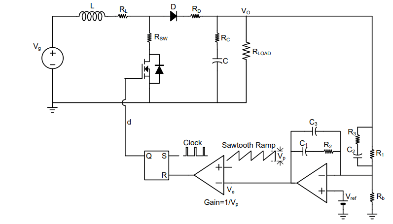
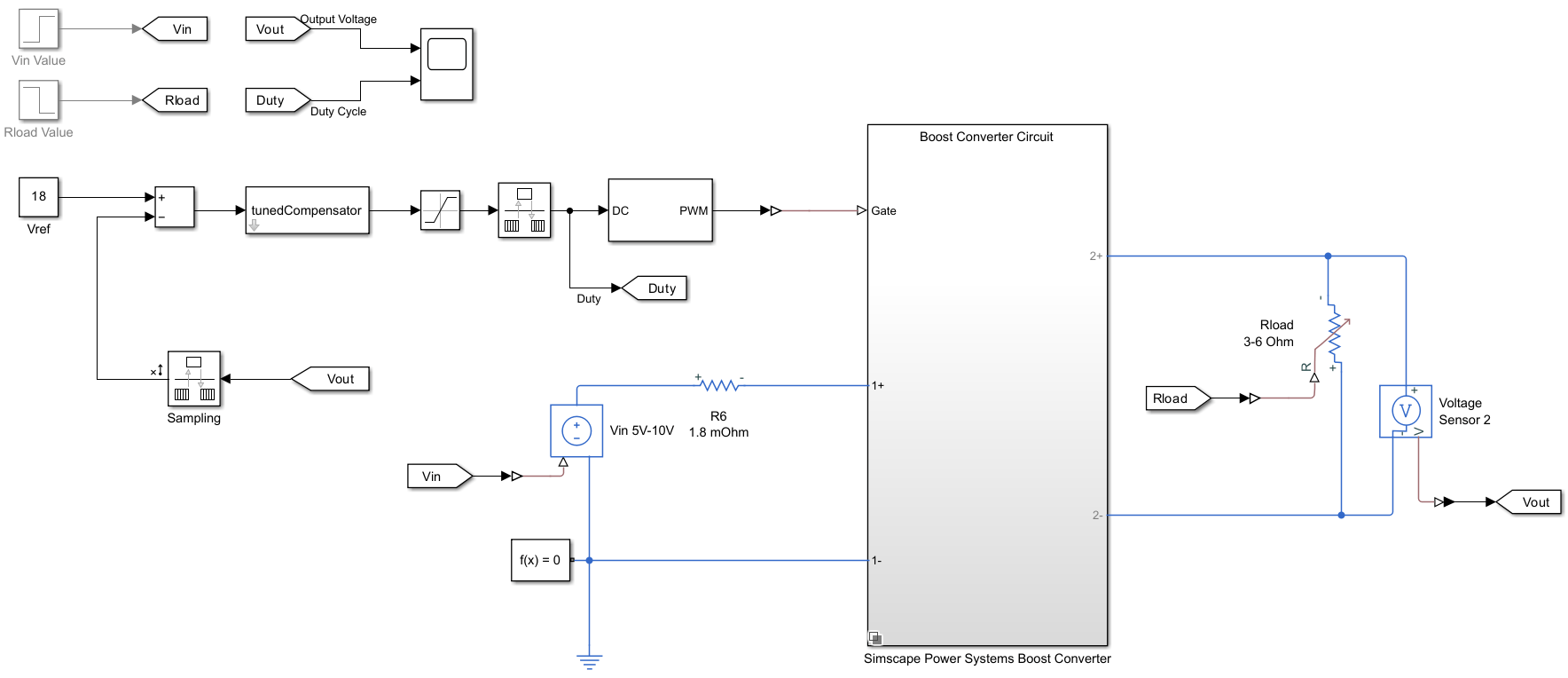
The power supply system consists of a voltage source, boost power train, load, feedback amplifier and pulse width modulator. The boost converter converts input voltage to output voltage . The output voltage is measured across the load , and is the current through the load. This conversion is controlled by the pulse duty cycle at the output of the pulse width modulator, which is in turn controlled by the feedback amplifier. The feedback amplifier senses the output voltage and attempts to make it a fixed multiple of the reference voltage , in response to changes in the source voltage, load current, and load resistance.
Boost Converter Model
Create a transfer function model for the boost converter with defined component values, at an operating point specified using the duty cycle and output voltage values observed in [2]. Here, use the getBoostConverterPlant helper function (available in the folder for this example) to set up this model. For more information, see Design Controller for Boost Converter Model Using Frequency Response Data (Simulink Control Design).
boostConverterPlant = getBoostConverterPlant();
boostConverterPlant.InputName = {'d'};
boostConverterPlant.OutputName = {'Vo'};
Tunable Control Architecture with Type-III Compensator
Now, set up a closed-loop system for the boost converter using a type-III compensator as a feedback amplifier and a simple gain block as the modulator gain, as shown in the following architecture diagram.
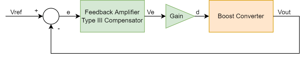
The objective is to tune the resistance (R1, R2, R3) and capacitance (C1, C2, C3) values of the type-III compensator which amplifies the error between the reference voltage and output voltage. A type-III compensator can increase phase in the mid-frequency range while improving both low and high frequency responses.
Create Tunable Linear System for Type-III Compensator
The type-III compensator structure is defined in the netlist file TypeIII_simple.sp. Run the getControlModel helper function, which uses a Linear Circuit Wizard block to parse the file and extract a tunable linear model. Configure the compensator using the configureTunableBlock helper function, and use a tunable gain in series to get the final controlBlock.
modelName = 'TypeIIICompensator';
load_system(modelName);
lcwBlock = [modelName,'/Linear Circuit Wizard'];
loadConfiguration(lcwBlock,'TypeIII_simpleCfg.mat');

% You can now open the mask of the Linear Circuit Wizard
% and examine or adjust the circuit configuration.

% Construct the symbolic model.
msblks.Circuit.packageCircuitAnalysis(lcwBlock,'Linear analysis');

compensator = getControlModel(lcwBlock,TypeIII_simpleCfgSymbolicModel);
compensator = configureTunableBlock(compensator);

K = realp('K',-1);
K.Minimum = -1.2;
K.Maximum = 0;

controlBlock = K*compensator;
controlBlock.InputName = {'e'};
controlBlock.OutputName = {'d'};
Connect Tunable and Fixed Blocks to Create Closed Loop System
eSum = sumblk('e = Vref - VoMeasured');
dSum = sumblk('VoMeasured = dVo + Vo');

closedLoopSystem = connect(controlBlock,boostConverterPlant,eSum,dSum,{'Vref','dVo'},'VoMeasured',{'e','d'});
Loop-Shaping Design
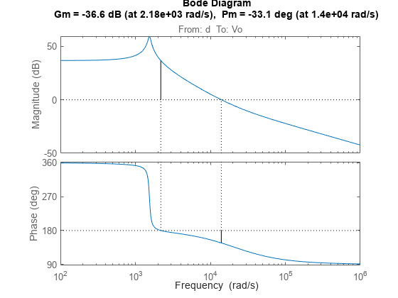
First, view the stability margins and frequency response of the open-loop boost converter plant.
figure;
margin(boostConverterPlant);
Design Requirements
Use the following design requirements to define a stable target loop shape:
Increase gain at low frequencies. Doing so improves the transient performance of reference voltage tracking and output voltage disturbance rejection and also reduces steady state error.
Add phase in middle frequencies to increase bandwidth (reduce response time) and achieve stability with positive gain and phase margins.
Reduce gain at high frequencies to make the closed loop system robust by attenuating oscillations in the control signal created by introduced harmonics and noisy measurements in the output voltage.
Use the helper function getTuningGoals to create the following tuning goal objects, which help you define constraints and objectives when you tune the system.
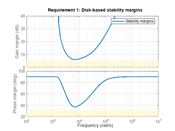
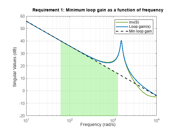
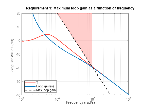
marginsGoal-TuningGoal.Margins(Control System Toolbox) with a gain margin constraint of 5 dB and phase margin constraint of 30 degrees. These constraints enforce stability and also help you visualize, usingviewGoal, how much uncertainty the loop can tolerate at different frequencies before going unstable.minLoopGainGoal-TuningGoal.MinLoopGain(Control System Toolbox) with an integral action gain profile and a bandwidth of 1 KHz. The constraint is enforced in the low frequency range (10 Hz to 200 Hz).maxLoopGainGoal-TuningGoal.MaxLoopGain(Control System Toolbox) with a double integrator gain profile and a roll-off of -40 dB/decade, enforced in the high frequency range (1.5 KHz to 15 KHz).
[marginsGoal, minLoopGainGoal, maxLoopGainGoal] = getTuningGoals();
Tune System
Now, use systune to tune the system, that is, compute the values of the tunable parameters (C1, C2, C3, R1, R2, R3, and K) such that the open loop response meets the desired design requirements.
First, create a systuneOptions object and adjust the values for the minimum decay rate and maximum spectral radius to suit tuning for high bandwidth loop shapes. Also, reduce the relative tolerance criteria for termination.
opts = systuneOptions;
opts.MinDecay = 1e-15;
opts.MaxRadius = 1e15;
opts.SoftTol = 1e-10;
Tune the system using systune, with the margin goals enforced as objectives (soft goals) and minimum and maximum loop gain goals enforces as constraints (hard goals). The tuning returns a converged result that satisfies the hard goals and optimizes the soft goals. The best achieved values for the soft and hard goals are both less than 1.
tunedClosedLoopSystem = systune(closedLoopSystem,marginsGoal,[minLoopGainGoal,maxLoopGainGoal],opts);
Final: Soft = 0.838, Hard = 0.99974, Iterations = 1064
Analyze Results
View Tuned System Results Against Desired Specifications
Create plots of the tuned system against the tuning goals to indicate how closely it meets the desired specifications. The shaded regions in each plot represent where the tuning goal is violated. The plots show that the constraints of tracking error and stability margins are met, while the objectives of minimum and maximum loop gains in specific frequency ranges are optimized.
viewGoal(marginsGoal,tunedClosedLoopSystem);
viewGoal(minLoopGainGoal,tunedClosedLoopSystem);
viewGoal(maxLoopGainGoal,tunedClosedLoopSystem);
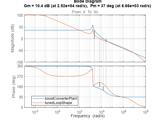
View Tuned Loop Shape and Stability Margins
The margin plot of the tuned open loop system indicates the bandwidth and robustness along with the achieved gain and phase margins.
tunedLoopShape = getLoopTransfer(tunedClosedLoopSystem,'d',-1);
figure;
margin(boostConverterPlant);
hold on;
margin(tunedLoopShape);
grid on;
legend('show','Location','best');
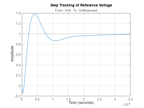
View Step Responses of Closed Loop System
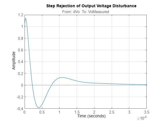
Step response plots of reference voltage tracking and output voltage disturbance tracking show that the response settles without any steady state error with an acceptably small settling time.
figure;
step(getIOTransfer(tunedClosedLoopSystem,'Vref','VoMeasured'));
title('Step Tracking of Reference Voltage');
grid on;
figure;
step(getIOTransfer(tunedClosedLoopSystem,'dVo','VoMeasured'));
title('Step Rejection of Output Voltage Disturbance');
grid on;
Tuned Component Values
Get the transfer function from the controller input e to the duty cycle d and display the tuned component values.
tunedCompensator = getIOTransfer(tunedClosedLoopSystem,'e','d','d');
showTunable(tunedCompensator);
C1 = 5.63e-08
-----------------------------------
C2 = 2.56e-09
-----------------------------------
C3 = 1e-11
-----------------------------------
K = -1.2
-----------------------------------
R1 = 2.37e+05
-----------------------------------
R2 = 1.12e+04
-----------------------------------
R3 = 1e+04
Simulation Results
Simulation Result with Tuned Controller
open_system("VoltageControlledBoostConverter.slx");Use an LTI System Block to implement the type-III compensator and simulate the model to examine the performance. The model uses the following disturbances:
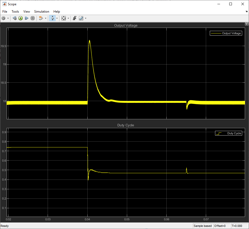
Line disturbance at t = 0.04 seconds, which increases the input voltage
Vinfrom 5 V to 10 V.Load disturbance at t = 0.065 seconds, which increases the load resistance
RLoadfrom 3 ohms to 6 ohms.
The results show that the tuned feedback amplifier rejects the line and load disturbances well.
References
[1] Lee, S. W. "Practical Feedback Loop Analysis for Voltage-Mode Boost Converter." Application Report No. SLVA633. Texas Instruments, January 2014. https://www.ti.com/lit/an/slva633/slva633.pdf.
[2] Ahmadi, Reza, and Mehdi Ferdowsi, "Modeling Closed-Loop Input and Output Impedances of DC-DC Power Converters Operating inside DC Distribution Systems." 2014 IEEE Applied Power Electronics Conference and Exposition - APEC 2014. IEEE, March 2014. https://ieeexplore.ieee.org/document/6803449.
You can also select a web site from the following list
Americas
- América Latina (Español)
- Canada (English)
- United States (English)
Europe
- Belgium (English)
- Denmark (English)
- Deutschland (Deutsch)
- España (Español)
- Finland (English)
- France (Français)
- Ireland (English)
- Italia (Italiano)
- Luxembourg (English)
- Netherlands (English)
- Norway (English)
- Österreich (Deutsch)
- Portugal (English)
- Sweden (English)
- Switzerland
- United Kingdom (English)
Asia Pacific
- Australia (English)
- India (English)
- New Zealand (English)
- 中国
- 日本Japanese (日本語)
- 한국Korean (한국어)