LDO Circuit Analysis Using Mixed Signal Analyzer

LDO

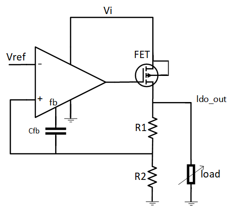
LDO is an analog circuit that maintains a constant output voltage relative to the input reference voltage, even with varying load current. The LDO schematic shown below comprises an Op-Amp, a pass-transistor (FET), and a resistive divider (R1, R2) in a feedback loop.

One of the important characteristics of the LDO is the load regulation. It is defined as the ability of the LDO to maintain a steady output with changes in the load current [1]. The worst case of the output voltage variation occurs as the load current transitions from zero to its maximum rated value or vice versa. Load regulation is a steady-state parameter. Therefore, the frequency components are ignored [1] and it is measured in simulation using the DC analysis in Cadence Virtuoso.

Phase margin is a dynamic parameter which represents the stability of the feedback loop in the LDO block. Phase margin is measured in simulation using stability analysis in Cadence Virtuoso.

LDO Simulation Data

To generate the LDO simulation data, simulate the LDO circuit in Cadence Virtuoso across various PVT (process, voltage, and temperature) corners. Save the metrics of interest such as load regulation, phase margin, and waveforms showing the transient behavior of the LDO. You can then extract the cadence simulation data into a mat file for further analysis in the Mixed Signal Analyzer app using the function adeinfo2msa.

Import Simulation Data in App

The LDO simulation data used in this example is saved in the mat file named ldo_test_Interactive.1.mat. Import the simulation data in the app.

mixedSignalAnalyzer('ldo_test_Interactive.1.mat')

The app opens and displays the list of simulation data imported from Cadence into the data panel of the app. Next, you can select any signal name and click the Display Waveform button in the toolstrip to visualize the signal. This image displays the waveform at output (ldo_out) of the LDO using the transient analysis data. You can also use MSA's cross-probing feature by clicking on a waveform in the plot window which highlights the row corresponding to the waveform's corner.

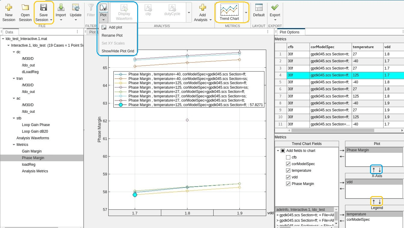
To visualize the phase margin metric, select the Phase Margin parameter in the data panel and click the Trend Chart button. You can also rename or rearrange the plots to customize them.

To save your plot customizations in a session mat file, click the Save Session button. This saves the session data in a mat file called LDO_Interactive.1.session.mat. To view the customizations saved in the session mat file, open the session.

mixedSignalAnalyzer('LDO_Interactive.1.session.mat')

Update Plots to Reflect Changes in Design Parameters

You can update the plots based on your customization when you change the design parameters to meet the design specifications.

In this example the minimum requirement on the LDO phase margin is 60 degrees. You can click on the points on the trend chart that violate the minimum phase margin requirement and observe that the corresponding rows get highlighted in the Plot Options table. It can be seen that all the points less than 60 degrees belong to the FF corner. You can change the design variable cfb to improve the phase margin and re-run the simulation to verify the results. First find out the value of cfb using the function call shown below.

cfb = adeGet("varName","cfb")

Next you can set a new value for cfb and re-run the simulation using the function calls shown below.

% Set variable value
adeSet("varName", "cfb", "varValue", "30f")
% Simulate
adeSim()

Generate a new mat file consisting of simulation results from the updated design.

 adeinfo2msa(runName='Interactive.2',metricsOnly=false,import2msa='false')

This creates a new mat file with the updated results called ldo_test_Interactive.2.mat.

You can update the app session by using the new simulation mat file and the session mat file from the previous section as input arguments.

msaSessionUpdate(sessionFileName='LDO_Interactive.1.session.mat', ... 
    sessionPath='./', updateMatFileName='ldo_test_Interactive.2.mat', ...
    reportType='pdf', reportFileName='LDO_Design_Report')

This also generates a report from the input arguments.

You can see that the LDO phase margin meets the minimum 60 degrees requirement at all corners after changing the cfb parameter.

Update Simulation Data from Cadence

You can also update the plots directly from Cadence without generating a simulation mat file. To do so,is by add the msaSessionUpdate function as a MATLAB® expression in the Outputs Setup in the Maestro view. At the end of the simulation, the Mixed Signal Analyzer app plots gets updated with new simulation data using the customizations from the session mat file, in this case, ldoSession.mat.

Reference

[1] Understanding the Terms and Definitions of LDO Voltage Regulators