Magnetometer Calibration

Ideal Magnetometers

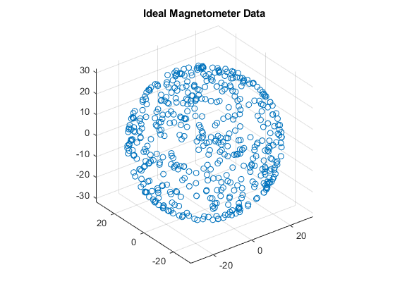
An ideal three-axis magnetometer measures magnetic field strength along orthogonal X, Y and Z axes. Absent any magnetic interference, magnetometer readings measure the Earth's magnetic field. If magnetometer measurements are taken as the sensor is rotated through all possible orientations, the measurements should lie on a sphere. The radius of the sphere is the magnetic field strength.

To generate magnetic field samples, use the imuSensor object. For these purposes it is safe to assume the angular velocity and acceleration are zero at each orientation.

N = 500;
rng(1);
acc = zeros(N,3);
av = zeros(N,3);
q = randrot(N,1); % uniformly distributed random rotations
imu = imuSensor('accel-mag');
[~,x] = imu(acc,av,q);
scatter3(x(:,1),x(:,2),x(:,3));
axis equal
title('Ideal Magnetometer Data');

Hard Iron Effects

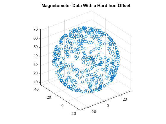
Noise sources and manufacturing defects degrade a magnetometer's measurement. The most striking of these are hard iron effects. Hard iron effects are stationary interfering magnetic noise sources. Often, these come from other metallic objects on the circuit board with the magnetometer. The hard iron effects shift the origin of the ideal sphere.

imu.Magnetometer.ConstantBias = [2 10 40];
[~,x] = imu(acc,av,q);
figure;
scatter3(x(:,1),x(:,2),x(:,3));
axis equal
title('Magnetometer Data With a Hard Iron Offset');

Soft Iron Effects

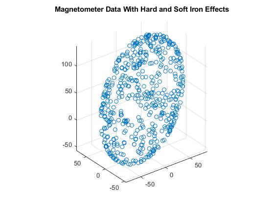
Soft iron effects are more subtle. They arise from objects near the sensor which distort the surrounding magnetic field. These have the effect of stretching and tilting the sphere of ideal measurements. The resulting measurements lie on an ellipsoid.

The soft iron magnetic field effects can be simulated by rotating the geomagnetic field vector of the IMU to the sensor frame, stretching it, and then rotating it back to the global frame.

nedmf = imu.MagneticField;
Rsoft = [2.5 0.3 0.5; 0.3 2 .2; 0.5 0.2 3];
soft = rotateframe(conj(q),rotateframe(q,nedmf)*Rsoft);

for ii=1:numel(q)
    imu.MagneticField = soft(ii,:);
    [~,x(ii,:)] = imu(acc(ii,:),av(ii,:),q(ii));
end
figure;
scatter3(x(:,1),x(:,2),x(:,3));
axis equal
title('Magnetometer Data With Hard and Soft Iron Effects');

Correction Technique

The magcal function can be used to determine magnetometer calibration parameters that account for both hard and soft iron effects. Uncalibrated magnetometer data can be modeled as lying on an ellipsoid with equation

In this equation R is a 3-by-3 matrix, b is a 1-by-3 vector defining the ellipsoid center, x is a 1-by-3 vector of uncalibrated magnetometer measurements, and is a scalar indicating the magnetic field strength. The above equation is the general form of a conic. For an ellipsoid, R must be positive definite. The magcal function uses a variety of solvers, based on different assumptions about R. In the magcal function, R can be assumed to be the identity matrix, a diagonal matrix, or a symmetric matrix.

The magcal function produces correction coefficients that take measurements which lie on an offset ellipsoid and transform them to lie on an ideal sphere, centered at the origin. The magcal function returns a 3-by-3 real matrix A and a 1-by-3 vector b. To correct the uncalibrated data compute

Here x is a 1-by-3 array of uncalibrated magnetometer measurements and m is the 1-by-3 array of corrected magnetometer measurements, which lie on a sphere. The matrix A has a determinant of 1 and is the matrix square root of R. Additionally, A has the same form as R : the identity, a diagonal, or a symmetric matrix. Because these kinds of matrices cannot impart a rotation, the matrix A will not rotate the magnetometer data during correction.

The magcal function also returns a third output which is the magnetic field strength . You can use the magnetic field strength to set the ExpectedMagneticFieldStrength property of ahrsfilter.

Using the magcal Function

Use the magcal function to determine calibration parameters that correct noisy magnetometer data. Create noisy magnetometer data by setting the NoiseDensity property of the Magnetometer property in the imuSensor. Use the rotated and stretched magnetic field in the variable soft to simulate soft iron effects.

imu.Magnetometer.NoiseDensity = 0.08;
for ii=1:numel(q)
    imu.MagneticField = soft(ii,:);
    [~,x(ii,:)] = imu(acc(ii,:),av(ii,:),q(ii));
end

To find the A and b parameters which best correct the uncalibrated magnetometer data, simply call the function as:

[A,b,expMFS]  = magcal(x);
xCorrected = (x-b)*A;

Plot the original and corrected data. Show the ellipsoid that best fits the original data. Show the sphere on which the corrected data should lie.

de = HelperDrawEllipsoid;
de.plotCalibrated(A,b,expMFS,x,xCorrected,'Auto');

The magcal function uses a variety of solvers to minimize the residual error. The residual error is the sum of the distances between the calibrated data and a sphere of radius expMFS.

r = sum(xCorrected.^2,2) - expMFS.^2;
E = sqrt(r.'*r./N)./(2*expMFS.^2);
fprintf('Residual error in corrected data : %.2f\n\n',E);

Residual error in corrected data : 0.01

You can run the individual solvers if only some defects need to be corrected or to achieve a simpler correction computation.

Offset-Only Computation

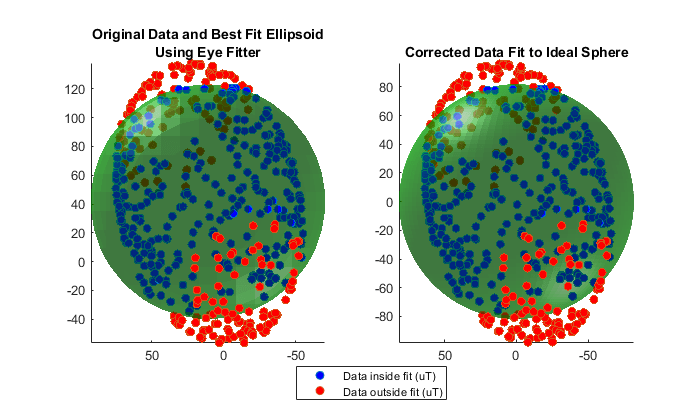
Many MEMS magnetometers have registers within the sensor that can be used to compensate for the hard iron offset. In effect, the (x-b) portion of the equation above happens on board the sensor. When only a hard iron offset compensation is needed, the A matrix effectively becomes the identity matrix. To determine the hard iron correction alone, the magcal function can be called this way:

[Aeye,beye,expMFSeye] = magcal(x,'eye');
xEyeCorrected = (x-beye)*Aeye;
[ax1,ax2] = de.plotCalibrated(Aeye,beye,expMFSeye,x,xEyeCorrected,'Eye');
view(ax1,[-1 0 0]);
view(ax2,[-1 0 0]);

Hard Iron Compensation and Axis Scaling Computation

For many applications, treating the ellipsoid matrix as a diagonal matrix is sufficient. Geometrically, this means the ellipsoid of uncalibrated magnetometer data is approximated to have its semiaxes aligned with the coordinate system axes and a center offset from the origin. Though this is unlikely to be the actual characteristics of the ellipsoid, it reduces the correction equation to a single multiply and single subtract per axis.

[Adiag,bdiag,expMFSdiag] = magcal(x,'diag');
xDiagCorrected = (x-bdiag)*Adiag;
[ax1,ax2] = de.plotCalibrated(Adiag,bdiag,expMFSdiag,x,xDiagCorrected,...
    'Diag');

Full Hard and Soft Iron Compensation

To force the magcal function to solve for an arbitrary ellipsoid and produce a dense, symmetric A matrix, call the function as:

[A,b] = magcal(x,'sym');

Auto Fit

The 'eye', 'diag', and 'sym' flags should be used carefully and the output values inspected. In some cases, there may be insufficient data for a high order ('diag' or 'sym') fit and a better set of correction parameters can be found using a simpler A matrix. The 'auto' fit option, which is the default, handles this situation.

Consider the case when insufficient data is used with a high order fitter.

xidx = x(:,3) > 100;
xpoor = x(xidx,:);
[Apoor,bpoor,mfspoor] = magcal(xpoor,'diag');

There is not enough data spread over the surface of the ellipsoid to achieve a good fit and proper calibration parameters with the 'diag' option. As a result, the Apoor matrix is complex.

disp(Apoor)

   0.0000 + 0.4722i   0.0000 + 0.0000i   0.0000 + 0.0000i
   0.0000 + 0.0000i   0.0000 + 0.5981i   0.0000 + 0.0000i
   0.0000 + 0.0000i   0.0000 + 0.0000i   3.5407 + 0.0000i

Using the 'auto' fit option avoids this problem and finds a simpler A matrix which is real, symmetric, and positive definite. Calling magcal with the 'auto' option string is the same as calling without any option string.

[Abest,bbest,mfsbest] = magcal(xpoor,'auto');
disp(Abest)

     1     0     0
     0     1     0
     0     0     1

Comparing the results of using the 'auto' fitter and an incorrect, high order fitter show the perils of not examining the returned A matrix before correcting the data.

de.compareBest(Abest,bbest,mfsbest,Apoor,bpoor,mfspoor,xpoor);

Calling the magcal function with the 'auto' flag, which is the default, will try all possibilities of 'eye', 'diag' and 'sym' searching for the A and b which minimizes the residual error, keeps A real, and ensures R is positive definite and symmetric.

Conclusion

The magcal function can give calibration parameters to correct hard and soft iron offsets in a magnetometer. Calling the function with no option string, or equivalently the 'auto' option string, produces the best fit and covers most cases.