Optimization Based Path Smoothing for Autonomous Vehicles

Open Live Script

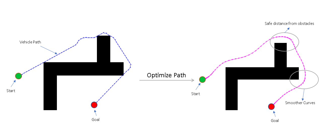
This example shows you how to optimize the path for a car-like robot by maintaining a smooth curvature and a safe distance from the obstacles in a parking lot.

In this example, you can use the optimizePath function along with the optimizePathOptions object to optimize a planned path. You can use any 2-D path planner like plannerRRT, plannerRRTStar, plannerAstar, plannerHybridAStar, etc. to plan a path from the entrance of the parking lot to a desired parking slot. In a parking lot like environment, the car often needs to take sharp turns and avoid obstacles like other cars, pillars, signboards, etc. The path generated by the path planners may not always be safe, easy to navigate, smooth, or kinematically feasible. In such situations path optimization becomes essential. The optimizePathOptions object has a large set of parameters and weights that you can tune to account for the environment and the vehicle constraints, the weights allows you to set their relative importance while optimizing the path.

Set Up Parking Lot Environment

Create a binaryOccupancyMap object from a parking lot map and set the map resolution as 3 cells/meter.

load("parkingMap.mat");
resolution = 3;
map = binaryOccupancyMap(map,resolution);

Visualize the map. The map contains the floor plan of a parking lot with some of the parking slots already occupied.

show(map)
title("Parking Lot Map")

Choose Parking Spot

The current position of the car at the entrance of the parking lot is taken as the start pose and a desired unoccupied parking slot is chosen as the goal pose of the vehicle.

Define the start and goal poses for the vehicle as [x y theta] vectors. x and y specify the position in meters, and theta specifies the orientation angle in radians.

startPose = [2 9 0];
goalPose = [27 18 pi/2];

Visualize the poses.

show(map)
hold on
quiver(startPose(1),startPose(2),cos(startPose(3)),sin(startPose(3)),2,...
       color=[0 0.75 0.23],LineWidth=2,...
       Marker="o",MarkerFaceColor=[0 0.75 0.23],MarkerSize=5,...
       DisplayName="Start Pose",ShowArrowHead="off");
quiver(goalPose(1),goalPose(2),cos(goalPose(3)),sin(goalPose(3)),2, ...
       color=[1 0 0],LineWidth=2,...
       Marker='o',MarkerFaceColor=[1 0 0],MarkerSize=5,...
       DisplayName="Goal Pose",ShowArrowHead="off");
legend(Location="southeast");
title("Start and Goal Poses in Parking Lot Map")
hold off

Path Planning

Create a validatorOccupancyMap state validator using the stateSpaceSE2 definition. Specify the map and the distance for interpolating and validating path segments.

validator = validatorOccupancyMap(stateSpaceSE2,map=map);
validator.ValidationDistance = 0.1;

Initialize the plannerHybridAStar object with the state validator object. Specify the MinTurningRadius and MotionPrimitiveLength properties of the planner.

planner = plannerHybridAStar(validator,MinTurningRadius=3,MotionPrimitiveLength=4);

Set default random number for repeatability.

rng("default");

Plan a path from the start pose to the goal pose.

refPath = plan(planner,startPose,goalPose);
path = refPath.States;

Visualize the planned path.

show(planner,Tree="off");
legend(Location="southeast");
hold off

Visualize the orientation of the vehicle.

plot(rad2deg(refPath.States(:,3)));
title("Orientation of Vehicle Along the Path in degrees")

Configure Path Optimization Parameters

The path generated by the planner is composed of continuous path segments, but the junctions might be discontinuous. These junctions can lead to abrupt changes in the steering angle. The path may also contain segments that add extra driving time. To avoid such motion, the path needs to be optimized and smoothed. The path sometimes are very close to the obstacles, which can be risky, especially for heavy vehicles like trucks.

Create Optimization Options

Create optimizePathOptions object to configure the behavior of the optimizePath function and the resulting path from it.

options = optimizePathOptions

options = 
optimizePathOptions

   Trajectory Parameters
                MaxPathStates: 200
           ReferenceDeltaTime: 0.3000
             MinTurningRadius: 1
                  MaxVelocity: 0.4000
           MaxAngularVelocity: 0.3000
              MaxAcceleration: 0.5000
       MaxAngularAcceleration: 0.5000

   Obstacle Parameters
         ObstacleSafetyMargin: 0.5000
       ObstacleCutOffDistance: 2.5000
    ObstacleInclusionDistance: 0.7500

   Solver Parameters
                 NumIteration: 4
           MaxSolverIteration: 15

   Weights
                   WeightTime: 10
             WeightSmoothness: 1000
       WeightMinTurningRadius: 10
               WeightVelocity: 100
        WeightAngularVelocity: 10
           WeightAcceleration: 10
    WeightAngularAcceleration: 10
              WeightObstacles: 50

Optimization options are grouped into four categories:

Trajectory Parameters
Obstacle Parameters
Solver Parameters
Weights

Trajectory Parameters

The trajectory parameters are used to specify the constraints of the vehicle while moving along the path like velocity, accelaration, turning radius, etc. They are soft limits which means that the solver might change them slightly while optimizing the path. Tune the following parameters,

MinTurningRadius - The turning radius of the vehicle. Increasing the MinTurningRadius will lead to larger path curvatures.
MaxVelocity - The maximum velocity that the vehicle can achieve. Changing this would modify the vehicle speed and trajectory time.
MaxAcceleration - The maximum accelartion possible for the vehicle.
ReferenceDeltaTime - Travel time between two consecutive poses. Increasing this would increase the vehicle speed.
MaxPathStates - Maximum number of poses allowed in path. Increasing this can give a smoother trajectory but might also increase the optimization time.

options.MinTurningRadius = 3; % meters
options.MaxVelocity = 5; % m/s
options.MaxAcceleration = 1; % m/s/s
options.ReferenceDeltaTime = 0.1; % second

separationBetweenStates = 0.2; % meters
numStates = refPath.pathLength/separationBetweenStates;
options.MaxPathStates = round(numStates);

Obstacle Parameters

The obstacle parameters specify the influence of the obstacles in the path. If there is a chance of the obstacles to move or their dimensions are not precisely known then you should keep the safety margin higher. In this example since most of the obstacles are lane markings and stationary parked vehicles, the safety margin can be smaller. Tune the following parameters,

ObstacleSafetyMargin - The safety margin that the path should maintain from the obstacles. Increasing the safety margin will make path safer and increase the distance from the obstacles.
ObstacleInclusionDistance - The obstacles within this distance from path will be included for the optimization.
ObstacleCutOffDistance - The obstacles beyond this distance from path will be ignored during optimization. This value must always be greater than obstacle inclusion distance.

For obstacles between the ObstacleInclusionDistance and ObstacleCutOffDistance the obstacles closest on the left and right sides between inclusion and cutoff distance are considered.

options.ObstacleSafetyMargin = 2; % meters
options.ObstacleInclusionDistance = 0.75; % meters
options.ObstacleCutOffDistance = 2.5; %i meters

Solver Parameters

The solver parameters specify the options for the solver used while optimizing the path. Higher values of these parameters improve the optimization results but also impact the optimization time, thus they should be tuned according to the need. Tune the following parameters,

NumIteration - Number of times solver is invoked during optimization, before each invocation the number of poses in the path are adjusted based on reference delta time.
MaxSolverIteration - Maximum number of iterations per solver invocation.

If path is already dense then the NumIteration can be reduced and MaxSolverIteration be increased. If path is sparse then NumIteration can be higher and MaxSolverIteration can be kept lower.

options.NumIteration = 4; 
options.MaxSolverIteration = 15;

Weights

The weights define the relative importance of various constraints discussed above. Since most of the constraints are soft limits, the weights decide how important a constraint is while optimizing the path. Tune the following weights,

WeightTime - Weight of the time component, increasing this would lead to shorter travel time and path.
WeightSmoothness - Increasing this weight will make the path smoother.
WeightMinTurningRadius - Increasing this will try to maintain the turning radius greater than the minimum value for most of the path.
WeightVelocity - Increasing this will ensure that the velocity constraints are more closely followed.
WeightObstacles - Increasing this will ensure that vehicle does not cross an obstacle.

options.WeightTime = 10;
options.WeightSmoothness = 1000;
options.WeightMinTurningRadius = 10;
options.WeightVelocity = 10;
options.WeightObstacles = 50;

Path Optimization

Use the optimizePath function to optimize the path generated by the planner according to optimization options defined above.

[optimizedPath,kineticInfo] = optimizePath(path,map,options);
drivingDir = sign(kineticInfo.Velocity);

Visualize the optimized path.

show(planner,Tree="off");
hold on
forwardMotion = optimizedPath(drivingDir==1,:);
reverseMotion = optimizedPath(drivingDir==-1,:);
quiver(forwardMotion(:,1),forwardMotion(:,2),cos(forwardMotion(:,3)),sin(forwardMotion(:,3)),...
    0.1,Color=[0 0.45 0.74],LineWidth=1,DisplayName="Optimized Forward Path");
quiver(reverseMotion(:,1),reverseMotion(:,2),cos(reverseMotion(:,3)),sin(reverseMotion(:,3)),...
    0.1,Color=[0.47 0.68 0.19],LineWidth=1,DisplayName="Optimized Reverse Path");
legend(Location="southeast");
title("Planned Path and Optimized Path")
hold off

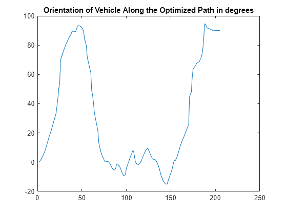
Plot the orientation of the vehicle along the optimized path.

plot(rad2deg(optimizedPath(:,3)))
title("Orientation of Vehicle Along the Optimized Path in degrees")

Tune Parameters with Live Controls

In the above section the path was optimized based on some preset parameter values. However, setting a good set of parameters can have a significant impact on the path.

In this section you can update the parameters using the sliders and visualize the impact they have on the optimized path. This will help you get a better understanding on how the parameters impact the final smooth path.

Trajectory Parameters

options.MinTurningRadius    =1.5; % m
options.MaxVelocity         =5; % m/s
options.MaxAcceleration     =1; % m/s/s

ReferenceDeltaTime is an important parameter and can have huge impact on the results.

options.ReferenceDeltaTime  =0.2; % s
separationBetweenStates     =0.2; % m
numStates = refPath.pathLength/separationBetweenStates;
options.MaxPathStates = round(numStates);

Obstacle Parameters

options.ObstacleSafetyMargin        =1.5;  % m
options.ObstacleCutOffDistance      =4;  % m
options.ObstacleInclusionDistance   =2;  % m

Solver Parameters

options.NumIteration        =2;
options.MaxSolverIteration  =8;

Weights

options.WeightTime              =200;
options.WeightSmoothness        =1000;
options.WeightMinTurningRadius  =140;
options.WeightVelocity          =230;
options.WeightObstacles         =320;

Optimize Path and Visualize

The new optimized path is plotted along with the previously generated and optimized path. This will help you compare the optimization results.

First plot the original path planned by the planner and the results of the previous optimization.

show(planner,Tree="off")
hold on
quiver(forwardMotion(:,1),forwardMotion(:,2),cos(forwardMotion(:,3)),sin(forwardMotion(:,3)),...
    0.1,Color=[0 0.45 0.74],LineWidth=1,DisplayName="Previous Optimized Forward Path");
quiver(reverseMotion(:,1),reverseMotion(:,2),cos(reverseMotion(:,3)),sin(reverseMotion(:,3)),...
    0.1,Color=[0.47 0.68 0.19],LineWidth=1,DisplayName="Previous Optimized Reverse Path");

Now optimize the path based on the new set of optimization options.

[optimizedPath,kineticInfo] = optimizePath(path,map,options);

Finally plot the new optimized path.

drivingDir = sign(kineticInfo.Velocity);

forwardMotion = optimizedPath(drivingDir==1,:);
reverseMotion = optimizedPath(drivingDir==-1,:);

quiver(forwardMotion(:,1),forwardMotion(:,2),cos(forwardMotion(:,3)),sin(forwardMotion(:,3)),...
    0.1,Color=[0.3 0.75 0.93],LineWidth=1,DisplayName="Optimized Forward Path");
quiver(reverseMotion(:,1),reverseMotion(:,2),cos(reverseMotion(:,3)),sin(reverseMotion(:,3)),...
    0.1,Color=[0.85 0.33 0.1],LineWidth=1,DisplayName="Optimized Reverse Path");

legend(Location="southeast");
title("Previous and Updated Optimized Path")

hold off

Reference

Rosmann, Christoph, Frank Hoffmann, and Torsten Bertram. “Kinodynamic Trajectory Optimization and Control for Car-like Robots.” In 2017 IEEE/RSJ International Conference on Intelligent Robots and Systems (IROS), 5681–86. Vancouver, BC: IEEE, 2017. https://doi.org/10.1109/IROS.2017.8206458.