工厂、仓库、销售分配模型：基于问题

此示例显示如何建立和求解混合整数线性规划问题。问题是在一组工厂、仓库和销售网点中找到最佳的生产和分销水平。有关基于求解器的方法，请参阅工厂、仓库、销售分配模型：基于求解器。

该示例首先为工厂、仓库和销售网点生成随机位置。请随意修改缩放参数 $N$ ，它不仅缩放生产和分销设施所在网格的大小，还缩放这些设施的数量，使得每个网格区域每种类型的设施密度与 $N$ 无关。

设施位置

对于缩放参数 $N$ 的给定值，假设存在以下内容：

$⌊ f N^{2} ⌋$ 工厂
$⌊ w N^{2} ⌋$ 仓库
$⌊ s N^{2} ⌋$ 销售网点

这些设施位于 $N$ 和 $x$ 方向 1 至 $y$ 之间的单独整数网格点上。为了使设施有单独的位置，您需要 $f + w + s \leq 1$ 。在此示例中，取 $N = 20$ 、 $f = 0.05$ 、 $w = 0.05$ 和 $s = 0.1$ 。

生产和发行

有工厂生产 $P$ 种产品。取 $P = 20$ 。

销售网点 $p$ 中每种产品 $s$ 的需求量为 $d (s, p)$ 。需求是在一定时间间隔内可以销售的数量。该模型的一个约束是需求得到满足，这意味着系统生产和分配的数量恰好是需求的数量。

每个工厂和每个仓库都有容量约束。

工厂 $p$ 生产的产品 $f$ 少于 $p c a p (f, p)$ 。
仓库 $w$ 的容量为 $w c a p (w)$ 。
在时间间隔内可以从仓库 $p$ 运输到销售网点的产品 $w$ 的数量小于 $t u r n (p) * w c a p (w)$ ，其中 $t u r n (p)$ 是产品 $p$ 的周转率。

假设每个销售网点仅从一个仓库接收供货。问题的一部分是确定销售网点到仓库的最便宜的映射。

成本

将产品从工厂运输到仓库，以及从仓库运输到销售网点的成本取决于设施之间的距离以及具体产品。如果 $d i s t (a, b)$ 是设施 $a$ 和 $b$ 之间的距离，那么在这两个设施之间运送产品 $p$ 的成本就是距离乘以运输成本 $t c o s t (p)$ ：

$d i s t (a, b) * t c o s t (p) .$

本例中的距离是网格距离，也称为 $L_{1}$ 距离。它是 $x$ 坐标和 $y$ 坐标的绝对差的总和。

工厂 $p$ 生产一单位产品 $f$ 的成本为 $p c o s t (f, p)$ 。

优化问题

给定一组设施位置以及需求和容量约束，找到：

每个工厂每种产品的生产水平
产品从工厂到仓库的配送时间表
产品从仓库到销售网点的配送时间表

这些数量必须确保满足需求并且总成本最小化。此外，每个销售网点都必须从一个仓库接收所有产品。

优化问题的变量和方程

控制变量，也就是您可以在优化中改变的变量，是

$x (p, f, w)$ = 从工厂 $p$ 运输到仓库 $f$ 的产品 $w$ 的数量
$y (s, w)$ = 二元变量，当销售网点 $s$ 与仓库 $w$ 关联时，取值为 1

要最小化的目标函数是

$\sum_{f} \sum_{p} \sum_{w} x (p, f, w) \cdot (p c o s t (f, p) + t c o s t (p) \cdot d i s t (f, w))$

$+ \sum_{s} \sum_{w} \sum_{p} (d (s, p) \cdot t c o s t (p) \cdot d i s t (s, w) \cdot y (s, w)) .$

约束包括

$\sum_{w} x (p, f, w) \leq p c a p (f, p)$ （工厂产能）。

$\sum_{f} x (p, f, w) = \sum_{s} (d (s, p) \cdot y (s, w))$ （需求得到满足）。

$\sum_{p} \sum_{s} \frac{d (s, p)}{t u r n (p)} \cdot y (s, w) \leq w c a p (w)$ （仓库容量）。

$\sum_{w} y (s, w) = 1$ （每个销售网点与一个仓库关联）。

$x (p, f, w) \geq 0$ （非负产量）。

$y (s, w) ϵ {0, 1}$ （二元变量 $y$ ）。

变量 $x$ 和 $y$ 线性出现在目标函数和约束函数中。由于 $y$ 仅限于整数值，因此该问题是混合整数线性规划 (MILP)。

生成随机问题：设施位置

设置 $N$ 、 $f$ 、 $w$ 、 $s$ 参数的值，并生成设施位置。

rng(1) % for reproducibility
N = 20; % N from 10 to 30 seems to work. Choose large values with caution.
N2 = N*N;
f = 0.05; % density of factories
w = 0.05; % density of warehouses
s = 0.1; % density of sales outlets

F = floor(f*N2); % number of factories
W = floor(w*N2); % number of warehouses
S = floor(s*N2); % number of sales outlets

xyloc = randperm(N2,F+W+S); % unique locations of facilities
[xloc,yloc] = ind2sub([N N],xyloc);

当然，设施随意选址是不现实的。此示例旨在展示解技术，而不是如何生成良好的设施位置。

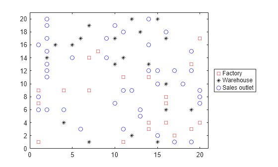
绘制设施。设施 1 至 F 为工厂，F+1 至 F+W 为仓库，F+W+1 至 F+W+S 为销售网点。

h = figure;
plot(xloc(1:F),yloc(1:F),'rs',xloc(F+1:F+W),yloc(F+1:F+W),'k*',...
    xloc(F+W+1:F+W+S),yloc(F+W+1:F+W+S),'bo');
lgnd = legend('Factory','Warehouse','Sales outlet','Location','EastOutside');
lgnd.AutoUpdate = 'off';
xlim([0 N+1]);ylim([0 N+1])

Figure contains an axes object. The axes object contains 3 objects of type line. One or more of the lines displays its values using only markers These objects represent Factory, Warehouse, Sales outlet.

生成随机容量、成本和需求

生成随机生产成本、产能、周转率和需求。

P = 20; % 20 products

% Production costs between 20 and 100
pcost = 80*rand(F,P) + 20;

% Production capacity between 500 and 1500 for each product/factory
pcap = 1000*rand(F,P) + 500;

% Warehouse capacity between P*400 and P*800 for each product/warehouse
wcap = P*400*rand(W,1) + P*400;

% Product turnover rate between 1 and 3 for each product
turn = 2*rand(1,P) + 1;

% Product transport cost per distance between 5 and 10 for each product
tcost = 5*rand(1,P) + 5;

% Product demand by sales outlet between 200 and 500 for each
% product/outlet
d = 300*rand(S,P) + 200;

这些随机的需求和能力可能会导致不可行的问题。换句话说，有时需求超出了生产和仓库容量的约束。如果您改变某些参数并得到一个不可行的问题，在解中您将得到一个 -2 的退出标志。

生成变量和约束

要开始指定问题，请生成距离数组 distfw(i,j) 和 distsw(i,j)。

distfw = zeros(F,W); % Allocate matrix for factory-warehouse distances
for ii = 1:F
    for jj = 1:W
        distfw(ii,jj) = abs(xloc(ii) - xloc(F + jj)) + abs(yloc(ii) ...
            - yloc(F + jj));
    end
end

distsw = zeros(S,W); % Allocate matrix for sales outlet-warehouse distances
for ii = 1:S
    for jj = 1:W
        distsw(ii,jj) = abs(xloc(F + W + ii) - xloc(F + jj)) ...
            + abs(yloc(F + W + ii) - yloc(F + jj));
    end
end

为优化问题创建变量。x 表示产量，连续变量，维度为 P×F×W。y 表示销售网点到仓库的二元分配，为 S×W 变量。

x = optimvar('x',P,F,W,'LowerBound',0);
y = optimvar('y',S,W,'Type','integer','LowerBound',0,'UpperBound',1);

现在创建约束。第一个约束是生产能力约束。

capconstr = sum(x,3) <= pcap';

下一个约束是每个销售网点都满足需求。

demconstr = squeeze(sum(x,2)) == d'*y;

每个仓库都有容量约束。

warecap = sum(diag(1./turn)*(d'*y),1) <= wcap';

最后，要求每个销售网点只连接到一个仓库。

salesware = sum(y,2) == ones(S,1);

创建问题和目标

创建一个优化问题。

factoryprob = optimproblem;

目标函数有三个部分。第一部分是生产成本的总和。

objfun1 = sum(sum(sum(x,3).*(pcost'),2),1);

第二部分是从工厂到仓库的运输费用总和。

objfun2 = 0;
for p = 1:P
    objfun2 = objfun2 + tcost(p)*sum(sum(squeeze(x(p,:,:)).*distfw));
end

第三部分是从仓库到销售网点的运输费用总和。

r = sum(distsw.*y,2); % r is a length s vector
v = d*(tcost(:));
objfun3 = sum(v.*r);

要最小化的目标函数是三部分的总和。

factoryprob.Objective = objfun1 + objfun2 + objfun3;

在问题中包含约束。

factoryprob.Constraints.capconstr = capconstr;
factoryprob.Constraints.demconstr = demconstr;
factoryprob.Constraints.warecap = warecap;
factoryprob.Constraints.salesware = salesware;

求解问题

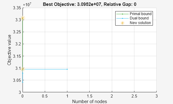
关闭迭代显示，这样您就不会得到数百行输出。包括一个绘图函数来监控解的进度。

opts = optimoptions("intlinprog",Display="off",...
    PlotFcn=@optimplotmilp);

调用求解器来寻找解。

[sol,fval,exitflag,output] = solve(factoryprob,Options=opts);

Figure Optimization Plot Function contains an axes object. The axes object with title Best Objective: 3.0952e+07, Relative Gap: 0, xlabel Number of nodes, ylabel Objective value contains 3 objects of type line. One or more of the lines displays its values using only markers These objects represent Primal bound, Dual bound, New solution.

if isempty(sol) % If the problem is infeasible or you stopped early with no solution
    disp('The solver did not return a solution.')
    return % Stop the script because there is nothing to examine
end

检查解

检查退出标志和解的不可行性。

exitflag

exitflag = 
    OptimalSolution

infeas1 = max(max(infeasibility(capconstr,sol)))

infeas1 = 
7.5943e-11

infeas2 = max(max(infeasibility(demconstr,sol)))

infeas2 = 
6.3545e-09

infeas3 = max(infeasibility(warecap,sol))

infeas3 = 
0

infeas4 = max(infeasibility(salesware,sol))

infeas4 = 
5.1625e-14

将解的 y 部分四舍五入为整数值。要了解为什么这些变量可能不完全是整数，请参阅有些“整数”解不是整数。

sol.y = round(sol.y); % get integer solutions

每个仓库关联多少个销售网点？请注意，在这种情况下，一些仓库有 0 个关联出口，这意味着这些仓库在最佳解中未被使用。

outlets = sum(sol.y,1)

outlets = 1×20

     2     0     3     2     2     2     3     2     3     2     1     0     0     3     4     3     2     3     2     1

绘制每个销售网点与其仓库之间的连接。

figure(h);
hold on
for ii = 1:S
    jj = find(sol.y(ii,:)); % Index of warehouse associated with ii
    xsales = xloc(F+W+ii); ysales = yloc(F+W+ii);
    xwarehouse = xloc(F+jj); ywarehouse = yloc(F+jj);
    if rand(1) < .5 % Draw y direction first half the time
        plot([xsales,xsales,xwarehouse],[ysales,ywarehouse,ywarehouse],'g--')
    else % Draw x direction first the rest of the time
        plot([xsales,xwarehouse,xwarehouse],[ysales,ysales,ywarehouse],'g--')
    end
end
hold off

title('Mapping of sales outlets to warehouses')

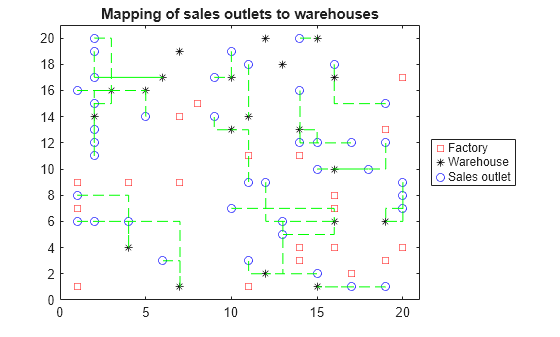
Figure contains an axes object. The axes object with title Mapping of sales outlets to warehouses contains 43 objects of type line. One or more of the lines displays its values using only markers These objects represent Factory, Warehouse, Sales outlet.

没有绿线的黑色*代表未使用的仓库。