拟合常微分方程 (ODE)
此示例说明如何以两种方式对数据进行 ODE 的参数拟合。第一种方式是直接对洛仑兹方程组的部分解进行恒速圆周轨迹拟合。洛仑兹方程组是著名的 ODE,高度依赖于初始参数。第二个示例说明如何修改洛仑兹方程组的参数,以拟合恒速圆周轨迹。您可以针对您的应用使用适当的方法,作为对数据进行微分方程拟合的模型。
洛仑兹方程组:定义和数值解
洛仑兹方程组是常微分方程组(请参阅洛仑兹方程组)。对于实数常量 ,方程组为
一个敏感系统的洛仑兹参数值是 。从 [x(0),y(0),z(0)] = [10,20,10] 开始启动系统,查看系统从时间 0 到 100 的演变。
sigma = 10;
beta = 8/3;
rho = 28;
f = @(t,a) [-sigma*a(1) + sigma*a(2); rho*a(1) - a(2) - a(1)*a(3); -beta*a(3) + a(1)*a(2)];
xt0 = [10,20,10];
[tspan,a] = ode45(f,[0 100],xt0);     % Runge-Kutta 4th/5th order ODE solver
figure
plot3(a(:,1),a(:,2),a(:,3))
view([-10.0 -2.0])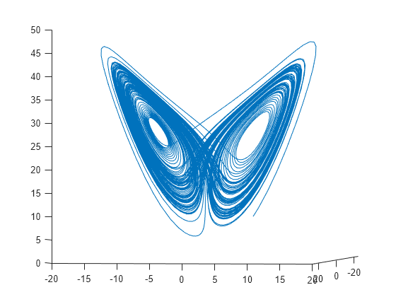
演变相当复杂。但在很短的时间区间内,它看起来有点像匀速圆周运动。绘制 [0,1/10] 时间区间内的解。
[tspan,a] = ode45(f,[0 1/10],xt0);     % Runge-Kutta 4th/5th order ODE solver
figure
plot3(a(:,1),a(:,2),a(:,3))
view([-30 -70])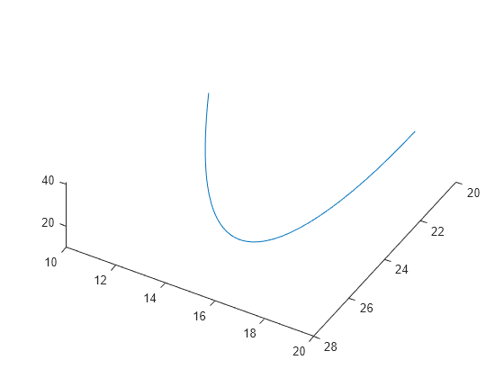
对 ODE 解进行圆周路径拟合
圆周轨迹的方程组有几个参数:
路径与 x-y 平面间的夹角
平面与 x 轴向倾角间的夹角
半径 R
速度 V
相对于时间 0 的时移 t0
空间 delta 中的三维位移
根据这些参数,可确定时间 xdata 的圆周轨迹的位置。
function f = fitlorenzfn(x,xdata)

theta = x(1:2);
R = x(3);
V = x(4);
t0 = x(5);
delta = x(6:8);
f = zeros(length(xdata),3);
f(:,3) = R*sin(theta(1))*sin(V*(xdata - t0)) + delta(3);
f(:,1) = R*cos(V*(xdata - t0))*cos(theta(2)) ...
    - R*sin(V*(xdata - t0))*cos(theta(1))*sin(theta(2)) + delta(1);
f(:,2) = R*sin(V*(xdata - t0))*cos(theta(1))*cos(theta(2)) ...
    - R*cos(V*(xdata - t0))*sin(theta(2)) + delta(2);
end
要求得洛仑兹方程组在 ODE 解的时间点处的最佳拟合圆周轨迹,请使用 lsqcurvefit。为了将参数保持在合理的范围内,可对各参数设置边界。
lb = [-pi/2,-pi,5,-15,-pi,-40,-40,-40];
ub = [pi/2,pi,60,15,pi,40,40,40];
theta0 = [0;0];
R0 = 20;
V0 = 1;
t0 = 0;
delta0 = zeros(3,1);
x0 = [theta0;R0;V0;t0;delta0];
[xbest,resnorm,residual] = lsqcurvefit(@fitlorenzfn,x0,tspan,a,lb,ub);
Local minimum possible.

lsqcurvefit stopped because the final change in the sum of squares relative to
its initial value is less than the value of the function tolerance.

<stopping criteria details>
绘制 ODE 解的时间点处的最佳拟合圆周点以及洛仑兹方程组的解。
soln = a + residual;
hold on
plot3(soln(:,1),soln(:,2),soln(:,3),"r")
legend("ODE Solution","Circular Arc")
hold off
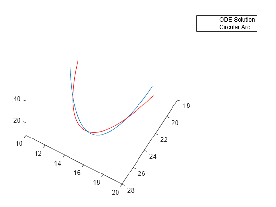
figure
plot3(a(:,1),a(:,2),a(:,3),"b.",MarkerSize=10)
hold on
plot3(soln(:,1),soln(:,2),soln(:,3),"rx",MarkerSize=10)
legend("ODE Solution","Circular Arc")
hold off

对圆弧进行 ODE 拟合
现在修改参数 ,使其与圆弧最佳拟合。为了更好地拟合,也允许初始点 [10,20,10] 发生改变。
为此,请使用 paramfun 函数,该函数采用 ODE 拟合的参数,并计算在时间 t 上的轨迹。
function pos = paramfun(x,tspan)

sigma = x(1);
beta = x(2);
rho = x(3);
xt0 = x(4:6);
f = @(t,a) [-sigma*a(1) + sigma*a(2); rho*a(1) - a(2) - a(1)*a(3); -beta*a(3) + a(1)*a(2)];
[~,pos] = ode45(f,tspan,xt0);
end
要找到最佳参数,可使用 lsqcurvefit 来最小化新计算的 ODE 轨迹和圆弧 soln 之差。
xt0 = zeros(1,6);
xt0(1) = sigma;
xt0(2) = beta;
xt0(3) = rho;
xt0(4:6) = soln(1,:);
[pbest,presnorm,presidual,exitflag,output] = lsqcurvefit(@paramfun,xt0,tspan,soln);
Local minimum possible.

lsqcurvefit stopped because the final change in the sum of squares relative to
its initial value is less than the value of the function tolerance.

<stopping criteria details>
确定这种优化对参数的改变程度。
fprintf("New parameters: %f, %f, %f",pbest(1:3))New parameters: 9.132446, 2.854998, 27.937986
fprintf("Original parameters: %f, %f, %f",[sigma,beta,rho])Original parameters: 10.000000, 2.666667, 28.000000
参数 sigma 和 beta 大约改变 10%。
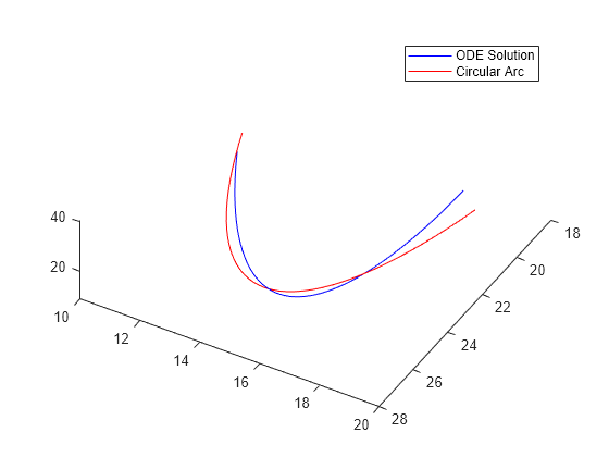
绘制修正后的解。
figure
hold on
odesl = presidual + soln;
plot3(odesl(:,1),odesl(:,2),odesl(:,3),"b")
plot3(soln(:,1),soln(:,2),soln(:,3),"r")
legend("ODE Solution","Circular Arc")
view([-30 -70])
hold off
ODE 拟合中的问题
如优化仿真或常微分方程中所述,优化器可能会因为数值 ODE 解中的固有噪声而遇到问题。如果您怀疑解不理想(例如,退出消息或退出标志指示解可能不准确),则可尝试更改有限差分运算。在本示例中,我们使用了更大的有限差分步长和中心有限差分。
options = optimoptions("lsqcurvefit",FiniteDifferenceStepSize=1e-4,...
    FiniteDifferenceType="central");
[pbest2,presnorm2,presidual2,exitflag2,output2] = ...
    lsqcurvefit(@paramfun,xt0,tspan,soln,[],[],options);
Local minimum possible.

lsqcurvefit stopped because the final change in the sum of squares relative to
its initial value is less than the value of the function tolerance.

<stopping criteria details>
在这一情况中,使用这些有限差分选项不能改进解。
disp([presnorm,presnorm2])
20.0637 20.0637