基于问题的离散化最优轨迹

打开实时脚本

此示例展示如何使用基于问题的方法求解离散化最佳轨迹问题。该轨迹具有恒定的重力、施加的力的限制并且没有空气阻力。解过程是在固定时间 $T$ 内求解最佳轨迹，并使用该解找到最佳 $T$ ，即最小化成本的时间。然后，该示例展示了如何考虑空气阻力，以及最后如何考虑物体消耗燃料时质量变化的影响。

与非离散化优化（例如示例使用优化变量拟合 ODE 参数）相比，离散化版本在求解常微分方程 (ODE) 时不那么准确。但是，离散化版本不受变步长 ODE 求解器中的噪声的影响，如优化仿真或常微分方程中所述。离散化版本也更容易定制，并且易于建模。最后，离散化版本可以利用优化过程中的自动微分；请参阅自动微分在基于问题的优化中的作用。

问题描述

问题是使用受控喷气机将物体在时间 $0$ 时的位置 $p_{0}$ 移动到时间 $T$ 时的位置 $p_{F}$ 。将位置表示为向量 $p (t)$ ，速度表示为向量 $v (t)$ ，将施加的加速度表示为向量 $a (t)$ 。在连续时间中，包括重力在内的运动方程是

$\frac{d p}{d t} = v (t)$

$\frac{d v}{d t} = a (t) + g * [0, 0, - 1]$ .

喷气发动机产生加速度 $a (t)$ 。由此产生的加速度增加了重力项。

喷气机可施加的最大加速度是 $A_{m a x} = 25$ 。

通过离散化时间来求解问题。将时间分成 $N$ 个大小为 $t = T / N$ 的相等间隔。时间步骤 $i$ 的位置是向量 $p (i)$ ，速度是向量 $v (i)$ ，施加的加速度是向量 $a (i)$ 。您可以制作一组相当准确地表示 ODE 模型的方程。一些近似运动方程是

$v (i) = v (i - 1) + t (a (i - 1) + g), i = 1 . . . N$

$p (i) = p (i - 1) + t (\frac{v (i - 1) + v (i)}{2}), i = 1 . . . N .$

上述方程使用二点（梯形法则）近似来积分速度，使用一点（欧拉）近似来积分加速度。如果将加速度 $a (i)$ 视为适用于时间间隔 $i$ 的中心，则积分方案就是加速度的中点规则。整体积分方案给出简单的方程：步骤 $i$ 处的位置和速度仅取决于步骤 $i - 1$ 处的位置、速度和加速度。该方程式也很容易根据空气阻力进行修改。

边界条件是 $p (0) = p_{0}$ 、 $p (N) = p_{F}$ 和 $v (0) = v (N) = [0, 0, 0]$ 。设定初始位置和最终位置。

p0 = [0 0 0];
pF = [5 10 3];

MATLAB ® 索引从 1 开始，而不是 0。为了更容易索引，将间隔数指定为 $N - 1$ ，并让位置和速度的索引从 $1$ 到 $N$ 而不是从 $0$ 到 $N$ 。通过此索引，加速度具有索引 $1$ 到 $N - 1$ 。

使用喷气发动机在时间 $t$ 内产生力 $a$ 的成本是 $‖ a ‖ t$ 。总成本是加速度范数乘以 $t$ 的总和。

$C o s t = \sum_{i = 1}^{N - 1} ‖ a (i) ‖ t .$

要将此成本转换为优化变量中的线性成本，请创建变量 $s (i)$ 和相关的二阶锥约束。

$\begin{array}{l} C o s t = \sum_{i = 1}^{N - 1} s (i) t \\ ‖ a (i) ‖ \leq s (i) . \end{array}$

施加额外的约束，即加速度的范数在所有时间步骤内都受常数 Amax 的限制。

$‖ a (i) ‖ \leq A m a x .$

这些约束也是二阶锥约束。因为约束是线性或者二阶锥约束，并且目标函数是线性的，所以 solve 调用 coneprog 求解器来求解问题。

本示例末尾的 setupproblem1 辅助函数创建了一个固定时间 T 的优化问题。代码将运动方程作为问题约束。该函数包括空气阻力参量；为具有空气阻力的模型设置 air = true。有关空气阻力的定义，请参阅包括空气阻力部分。

施加的加速度 $a$ 是问题中的主要优化变量。正如 Vanderbei [1] 所建议的，该问题不需要将速度 v 和位置 p 作为优化变量。您可以从运动方程和施加的加速度 $a$ 的值推导出它们的值。对于 N 步骤， $a$ 的尺寸为 N – 1 x 3。该问题还包括向量变量 s 作为允许线性目标函数的优化变量。

求解 T = 20 的问题

创建并求解时间 $T = 20$ 的轨迹问题。为了保证这个数值敏感问题的可靠性，将最优容差设置为 1e-9。

[trajprob,p] = setupproblem1(20);

该问题的默认求解器是什么？

defaultsolver = solvers(trajprob)

defaultsolver = 
"coneprog"

设置 coneprog 求解器的选项并求解问题。

opts = optimoptions(defaultsolver,Display="none",OptimalityTolerance=1e-9);
[sol,fval,eflag,output] = solve(trajprob,Options=opts)

sol = struct with fields:
    a: [49×3 double]
    s: [49×1 double]

fval = 192.2812

eflag = 
    OptimalSolution

output = struct with fields:
           iterations: 12
    primalfeasibility: 4.4823e-10
      dualfeasibility: 3.3916e-09
           dualitygap: 3.2421e-11
            algorithm: 'interior-point'
         linearsolver: 'augmented'
              message: 'Optimal solution found.'
               solver: 'coneprog'

通过调用 plottrajandaccel 辅助函数绘制加速度的轨迹和范数。

N = 50;
plottrajandaccel(sol,p,p0,pF)

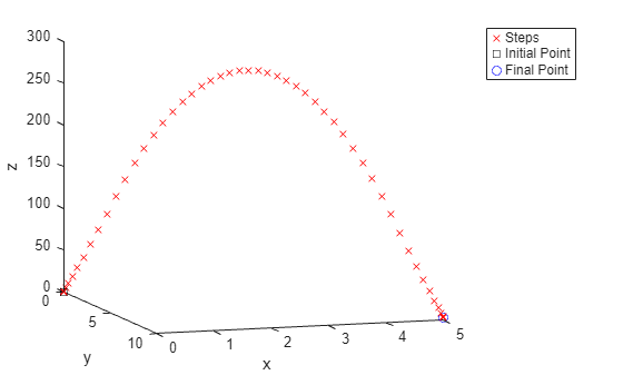
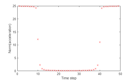
Figure contains an axes object. The axes object with xlabel x, ylabel y contains 3 objects of type line. One or more of the lines displays its values using only markers These objects represent Steps, Initial Point, Final Point.

Figure contains an axes object. The axes object with xlabel Time step, ylabel Norm(acceleration) contains a line object which displays its values using only markers.

加速度在开始和结束时接近最大值，在中间时接近于零。这种加速度要么最大要么为 0 的解被称为“bang-bang”。

寻找最小成本

什么时候 $T$ 会导致成本最小？对于太小的时间，例如 $T = 1$ ，问题是不可行的，意味着它没有解。

myprob = setupproblem1(1);
opts.Display = "RawMT"; % To see the solution status
[solm,fvalm,eflagm,outputm] = solve(myprob,Options=opts);

Solving problem using coneprog.
Problem is infeasible.

时间 1.5 给出了一个可行问题。

myprob = setupproblem1(1.5);
[solm,fvalm,eflagm,outputm] = solve(myprob,Options=opts);

Solving problem using coneprog.
Optimal solution found.

tomin 辅助函数设置了一个时间为 T 的问题，然后调用 solve 来计算解的成本。在 tomin 上调用 fminbnd 来找到区间 $1.5 \leq T \leq 10$ 中的最佳时间（可能成本最低）。

[Tmin,Fmin] = fminbnd(@(T)tomin(T,false),1.5,10)

Tmin = 1.9517

Fmin = 24.6095

获取最佳时间 Tmin 的轨迹。

[minprob,p] = setupproblem1(Tmin);
sol = solve(minprob,Options=opts);

Solving problem using coneprog.
Optimal solution found.

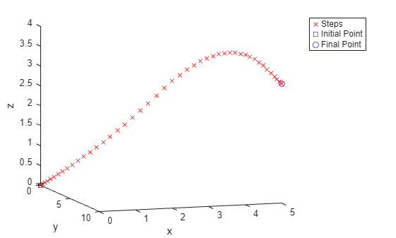
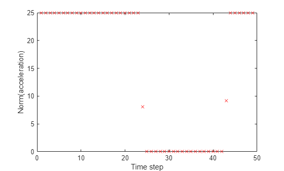
绘制最小化轨迹和加速度。

plottrajandaccel(sol,p,p0,pF)

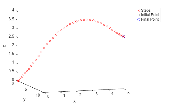
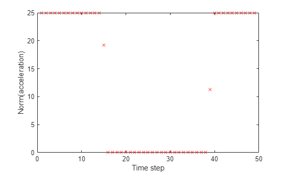
Figure contains an axes object. The axes object with xlabel Time step, ylabel Norm(acceleration) contains a line object which displays its values using only markers.

最小化解更接近于“bang-bang”解：除了两个值之外，加速度都是最大值或零。

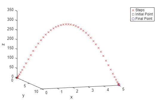
绘制非最小化轨迹

绘制不同时间的轨迹。

figure
hold on
options = optimoptions("coneprog",Display="none",OptimalityTolerance=1e-9);
g = [0 0 -9.81];
for i = 1:10
    T = 2*i;
    t = T/N;
    prob = setupproblem1(T);
    sol = solve(prob,"Options",options);
    asol = sol.a;
    vsol = cumsum([[0 0 0];t*(asol+repmat(g,size(asol,1),1))]);
    N = size(vsol,1);
    np = 2:N;
    n0 = 1:(N-1);
    psol = cumsum([p0;t*(vsol(np,:) + vsol(n0,:))/2]);
    plot3(psol(:,1),psol(:,2),psol(:,3),'rx',"Color",[256-25*i 20*i 25*i]/256)
end
view([18 -10])
xlabel("x")
ylabel("y")
zlabel("z")
legend("T = 2","T = 4","T = 6","T = 8","T = 10","T = 12","T = 14","T = 16","T = 18","T = 20")
hold off

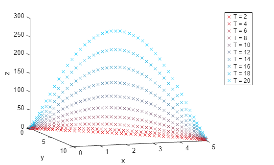
Figure contains an axes object. The axes object with xlabel x, ylabel y contains 10 objects of type line. One or more of the lines displays its values using only markers These objects represent T = 2, T = 4, T = 6, T = 8, T = 10, T = 12, T = 14, T = 16, T = 18, T = 20.

最短时间（2）在这个尺度上具有近乎直线的轨迹。时间越长，相对直线路径的变化就越大，其中 $T = 20$ 的路径达到接近 300 的高度。

包括空气阻力

改变模型动力学以包含空气阻力。线性空气阻力在时间 $t$ 之后使速度改变 $\exp (- t)$ 倍。运动方程变成

$v (i) = v (i - 1) \exp (- t) + t (a (i - 1) + g)$

$\begin{array}{l} p (i) = p (i - 1) + t (\frac{v (i - 1) + v (i)}{2}) \\ = p (i - 1) + t (\frac{1 + \exp (- t)}{2}) v (i - 1) + t^{2} \frac{a (i - 1) + g}{2} . \end{array}$

setupproblem1(T,air) 函数中针对 air = true 的问题表示在定义速度约束的线和定义位置约束的线中都有 exp(-t) 的因子：

vcons(2:N,:) = v(2:N,:) == v(1:(N-1),:)*exp(-t) + t*(a(1:(N-1),:) + repmat(g,N-1,1));
pcons(2:N,:) = p(2:N,:) == p(1:(N-1),:) + t*(1+exp(-t))/2*v(1:(N-1),:) + t^2/2*(a(1:(N-1),:) + repmat(g,N-1,1));

找到求解空气阻力问题的最佳时间。

[Tmin2,Fmin2] = fminbnd(@(T)tomin(T,true),1.5,10)

Tmin2 = 1.9398

Fmin2 = 28.7967

最优时间仅比没有空气阻力的问题中的时间略低（1.94 比 1.95），但成本 Fmin 高出约 17%（28.8 比 24.6）。

compartable = table([Tmin;Tmin2],[Fmin;Fmin2],'VariableNames',["Time" "Cost"],'RowNames',["Original" "Air Resistance"])

compartable=2×2 table
                       Time      Cost 
                      ______    ______

    Original          1.9517    24.609
    Air Resistance    1.9398    28.797

绘制具有空气阻力的最优解的轨迹和加速度。

[minprob,p] = setupproblem1(Tmin2,true);
sol = solve(minprob,Options=opts);

Solving problem using coneprog.
Optimal solution found.

plottrajandaccel(sol,p,p0,pF)

Figure contains an axes object. The axes object with xlabel Time step, ylabel Norm(acceleration) contains a line object which displays its values using only markers.

由于空气阻力，零加速度的时间转移到较晚的时间步骤并且更短。然而，解仍然几乎是“bang-bang”。

扩展模型以包含可变质量

喷气发动机通过排出物质来运转。如果将喷气推进过程中质量减小的影响考虑在内，运动方程就不再适合二阶锥问题框架。这个问题变得更难以用数字方式求解，导致解时间更长且答案更不准确。

更改模型以包含施加的力 $F (t)$ 和质量 $m (t)$ 。净加速度为

$a (t) = F (t) / m (t) + g [0, 0, - 1]$ .

质量变化率为

$\frac{d m}{d t} = - r ‖ F (t) ‖,$

其中， $r$ 是一个常量。

假设 $m (0) = 2$ 、 $r = 1 / 1000$ ，最大力量是 $F_{m a x} = 50$ 。这些假设意味着，在时间 0 时，施加的最大加速度是 $F_{m a x} / m (0) = 25$ ，与前一个模型中的最大加速度相同。

setupproblemfuel1 函数根据这些方程和参数创建问题。对于此变质量模型实例，不包括空气阻力。

[trajprob,p] = setupproblemfuel1(20);

由此产生的问题的默认求解器是什么？

defaultsolver = solvers(trajprob)

defaultsolver = 
"fmincon"

fmincon 求解器需要一个初始点。尝试 T = 20 的随机初始点。

rng default
y0 = randn(49,3);
x0.F = y0;

指定求解器在进行过程中生成图表的选项，并允许比默认值更多的函数计算和迭代。尝试将 StepTolerance 从默认的 1e-10 减少到 1e-11 以获得更高的准确性。

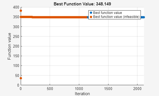
opts = optimoptions(defaultsolver,Display="none",PlotFcn="optimplotfvalconstr",...
    MaxFunctionEvaluations=1e5,MaxIterations=1e4,StepTolerance=1e-11);

调用求解器。

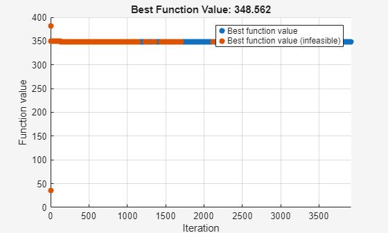
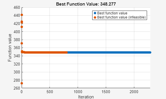
[sol,fval,eflag,output] = solve(trajprob,x0,Options=opts)

Figure Optimization Plot Function contains an axes object. The axes object with title Best Function Value: 348.149, xlabel Iteration, ylabel Function value contains 2 objects of type scatter. These objects represent Best function value, Best function value (infeasible).

sol = struct with fields:
    F: [49×3 double]

fval = 348.1493

eflag = 
    StepSizeBelowTolerance

output = struct with fields:
              iterations: 2393
               funcCount: 8148
         constrviolation: 2.7960e-12
                stepsize: 1.8893e-11
               algorithm: 'interior-point'
           firstorderopt: 0.0719
            cgiterations: 76125
                 message: 'Local minimum possible. Constraints satisfied.↵↵fmincon stopped because the size of the current step is less than↵the value of the step size tolerance and constraints are ↵satisfied to within the value of the constraint tolerance.↵↵<stopping criteria details>↵↵Optimization stopped because the relative changes in all elements of x are↵less than options.StepTolerance = 1.000000e-11, and the relative maximum constraint↵violation, 1.474630e-15, is less than options.ConstraintTolerance = 1.000000e-06.'
            bestfeasible: [1×1 struct]
     objectivederivative: "reverse-AD"
    constraintderivative: "reverse-AD"
                  solver: 'fmincon'

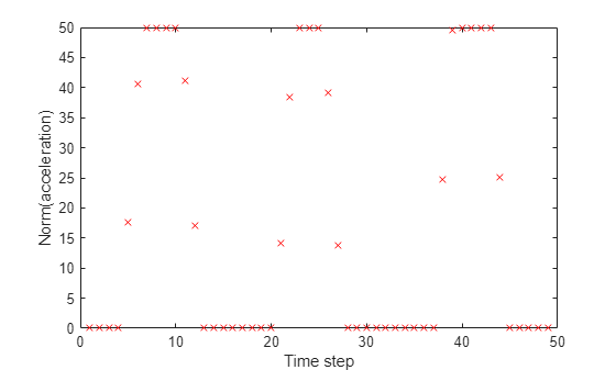
绘制轨迹和加速度。plottrajandaccel 函数使用解方案结构体中 a 字段的值，因此首先将解从 F 字段复制到 a 字段。

sol.a = sol.F;
plottrajandaccel(sol,p,p0,pF)

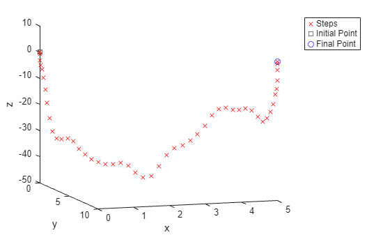
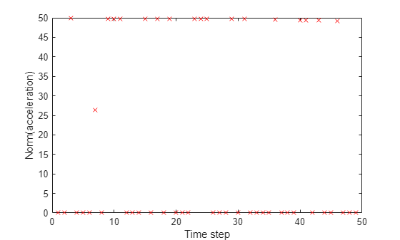
Figure contains an axes object. The axes object with xlabel Time step, ylabel Norm(acceleration) contains a line object which displays its values using only markers.

通过增加可变加速度的成本实现平滑解

施加的力本质上是“砰砰”的，但力却具有振荡行为。范德贝[1]将这种行为称为“响铃”。为了消除振铃，请增加一些振荡加速度的成本，然后再次求解。setupproblemfuel2 辅助函数在目标函数中包含一个附加项 t*1e-4*sum(diff(fnorm).^2，它对加速度范数的变化进行惩罚：

 % Add cost for acceleration changes
 trajectoryprob.Objective = sum(fnorm)*t + t*1e-4*sum(diff(fnorm).^2);

再次求解问题。

[trajprob,p] = setupproblemfuel2(20);
[sol,fval,eflag,output] = solve(trajprob,x0,Options=opts)

Figure Optimization Plot Function contains an axes object. The axes object with title Best Function Value: 348.562, xlabel Iteration, ylabel Function value contains 2 objects of type scatter. These objects represent Best function value, Best function value (infeasible).

sol = struct with fields:
    F: [49×3 double]

fval = 348.5616

eflag = 
    StepSizeBelowTolerance

output = struct with fields:
              iterations: 3755
               funcCount: 7927
         constrviolation: 3.2683e-11
                stepsize: 1.6872e-10
               algorithm: 'interior-point'
           firstorderopt: 0.1728
            cgiterations: 46335
                 message: 'Local minimum possible. Constraints satisfied.↵↵fmincon stopped because the size of the current step is less than↵the value of the step size tolerance and constraints are ↵satisfied to within the value of the constraint tolerance.↵↵<stopping criteria details>↵↵Optimization stopped because the relative changes in all elements of x are↵less than options.StepTolerance = 1.000000e-11, and the relative maximum constraint↵violation, 1.723720e-14, is less than options.ConstraintTolerance = 1.000000e-06.'
            bestfeasible: [1×1 struct]
     objectivederivative: "reverse-AD"
    constraintderivative: "reverse-AD"
                  solver: 'fmincon'

使用 sol.F 数据绘制轨迹和加速度。

sol.a = sol.F;
plottrajandaccel(sol,p,p0,pF)

Figure contains an axes object. The axes object with xlabel Time step, ylabel Norm(acceleration) contains a line object which displays its values using only markers.

提供更好的起点

大部分振铃已消失，但解仍然具有一个以上的零力间隔。

指定不同的初始点可能会得到更令人满意的解。为了使求解器在中间时间具有较小的加速度，请将索引 10 到 40 的初始点指定为等于 0，将索引 1 到 9 和 41 到 49 的初始点指定为等于 20。在初始点添加一些随机噪声。

rng default
y0 = 20*ones(49,3);
y0(10:40,:) = 0;
y0 = y0 + randn(size(y0));
x0.F = y0;

从这个新的点出发求解问题。

[sol,fval,eflag,output] = solve(trajprob,x0,Options=opts)

Figure Optimization Plot Function contains an axes object. The axes object with title Best Function Value: 348.277, xlabel Iteration, ylabel Function value contains 2 objects of type scatter. These objects represent Best function value, Best function value (infeasible).

sol = struct with fields:
    F: [49×3 double]

fval = 348.2770

eflag = 
    StepSizeBelowTolerance

output = struct with fields:
              iterations: 1653
               funcCount: 5422
         constrviolation: 7.6383e-14
                stepsize: 2.2832e-11
               algorithm: 'interior-point'
           firstorderopt: 0.0318
            cgiterations: 26724
                 message: 'Local minimum possible. Constraints satisfied.↵↵fmincon stopped because the size of the current step is less than↵the value of the step size tolerance and constraints are ↵satisfied to within the value of the constraint tolerance.↵↵<stopping criteria details>↵↵Optimization stopped because the relative changes in all elements of x are↵less than options.StepTolerance = 1.000000e-11, and the relative maximum constraint↵violation, 6.578331e-17, is less than options.ConstraintTolerance = 1.000000e-06.'
            bestfeasible: [1×1 struct]
     objectivederivative: "reverse-AD"
    constraintderivative: "reverse-AD"
                  solver: 'fmincon'

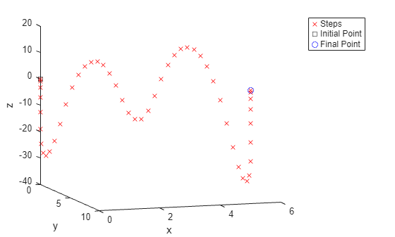
绘制轨迹和加速度。

sol.a = sol.F;
plottrajandaccel(sol,p,p0,pF)

Figure contains an axes object. The axes object with xlabel Time step, ylabel Norm(acceleration) contains a line object which displays its values using only markers.

该解似乎令人满意：它本质上是“砰砰”加速，只有一个施加加速度的零间隔。

物体旅程结束时，最初的 2 个质量剩下多少？

T = 20;
N = 50;
t = T/N;
fnorm = zeros(N-1,1);
r = 1/1000;
for i = 1:length(fnorm)
    fnorm(i) = norm(sol.F(i,:));
end
m = 2 - r*t*sum(fnorm)

m = 1.6518

在这个减小的质量下，最大施加加速度是多少？

Fmax = 50;
Fmax/m

ans = 30.2700

当模型包含变质量的影响时，轨迹期间施加的最大加速度从 25 变为 30。

包括空气阻力和可变质量

在模型中再次考虑空气阻力。在这种情况下，setupproblemfuel2 辅助函数使用 fcn2optimexpr 调用 airResistance 辅助函数来评估有空气阻力的速度。使用单独的函数编写 for 循环，然后使用 fcn2optimexpr 调用该函数，可以产生更高效的问题。有关详细信息，请参阅创建 for 循环进行静态分析和优化表达式的静态分析。

[trajprob2,p] = setupproblemfuel2(20,true);

根据之前考虑空气阻力的模型结果，将初始零力区间设定得较晚：15 到 45，而不是 10 到 40。

rng default
y0 = 20*ones(49,3);
y0(15:45,:) = 0;
y0 = y0 + randn(size(y0));
x0.F = y0;

求解。

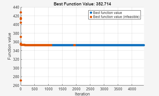
[sol2,fval2,eflag2,output2] = solve(trajprob2,x0,Options=opts)

Figure Optimization Plot Function contains an axes object. The axes object with title Best Function Value: 352.714, xlabel Iteration, ylabel Function value contains 2 objects of type scatter. These objects represent Best function value, Best function value (infeasible).

sol2 = struct with fields:
    F: [49×3 double]

fval2 = 352.7138

eflag2 = 
    StepSizeBelowTolerance

output2 = struct with fields:
              iterations: 6686
               funcCount: 12620
         constrviolation: 2.1938e-13
                stepsize: 1.5226e-11
               algorithm: 'interior-point'
           firstorderopt: 0.2178
            cgiterations: 93737
                 message: 'Local minimum possible. Constraints satisfied.↵↵fmincon stopped because the size of the current step is less than↵the value of the step size tolerance and constraints are ↵satisfied to within the value of the constraint tolerance.↵↵<stopping criteria details>↵↵Optimization stopped because the relative changes in all elements of x are↵less than options.StepTolerance = 1.000000e-11, and the relative maximum constraint↵violation, 1.532271e-15, is less than options.ConstraintTolerance = 1.000000e-06.'
            bestfeasible: [1×1 struct]
     objectivederivative: "reverse-AD"
    constraintderivative: "reverse-AD"
                  solver: 'fmincon'

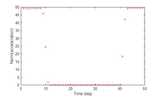
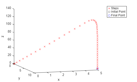
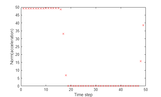
sol2.a = sol2.F;
plottrajandaccel(sol2,p,p0,pF)

Figure contains an axes object. The axes object with xlabel Time step, ylabel Norm(acceleration) contains a line object which displays its values using only markers.

剩余燃料的质量是多少？

for i = 1:length(fnorm)
    fnorm(i) = norm(sol2.F(i,:));
end
m2 = 2 - r*t*sum(fnorm)

m2 = 1.6474

在这个减小的质量下，最大施加加速度是多少？

Fmax/m2

ans = 30.3517

空气阻力的加入不会显著改变燃料的消耗。该轨迹似乎利用了空气阻力来帮助物体减慢速度，因此物体在旅程的最后阶段并不需要消耗太多燃料来减速。注意有空气阻力的弹道最大高度在 130 以下，而无空气阻力的弹道最大高度在 300 左右。在当前参数下，空气阻力会对轨迹产生明显影响，但不会改变燃料消耗。

参考资料

[1] Vanderbei, R. J."Case Studies in Trajectory Optimization:Trains, Planes, and Other Pastimes."Optimization and Engineering 2, 215–243 (2001).Available at https://vanderbei.princeton.edu/tex/trajopt/trajopt.pdf.

辅助函数

以下代码创建 setupproblem1 辅助函数。

function [trajectoryprob,p] = setupproblem1(T,air)
    if nargin == 1
        air = false;
    end
    N = 50;
    g = [0 0 -9.81];
    p0 = [0 0 0];
    pF = [5 10 3];
    Amax = 25;
    t = T/N;
    a = optimvar("a",N-1,3,"LowerBound",-Amax,"UpperBound",Amax);
    v = optimexpr(N,3);
    trajectoryprob = optimproblem;
    s = optimvar("s",N-1,"LowerBound",0,"UpperBound",3*Amax);
    trajectoryprob.Objective = sum(s)*t;
    scons = optimconstr(N-1);
    for i = 1:(N-1)
        scons(i) = norm(a(i,:)) <= s(i);
    end
    acons = optimconstr(N-1);
    for i = 1:(N-1)
        acons(i) = norm(a(i,:)) <= Amax;
    end
    np = 2:N;
    n0 = 1:(N-1);
    v0 = [0 0 0];
    if air
        v(1, :) = v0;
        for i = 2:N
            v(i,:) = v(i-1,:)*exp(-t) + t*(a(i-1,:) + g);
        end
    else
        gbig = repmat(g,size(a,1),1);
        v = cumsum([v0; t*(a + gbig)]);
    end
    p = cumsum([p0;t*(v(np,:) + v(n0,:))/2]); % Independent of "air"
    endcons = v(N,:) == [0 0 0];
    pcons2 = p(N,:) == pF;
    trajectoryprob.Constraints.acons = acons;
    trajectoryprob.Constraints.scons = scons;
    trajectoryprob.Constraints.endcons = endcons;
    trajectoryprob.Constraints.pcons2 = pcons2;
end

以下代码创建 plottrajandaccel 辅助函数。

function plottrajandaccel(sol,p,p0,pF)
figure
psol = evaluate(p, sol);
plot3(psol(:,1),psol(:,2),psol(:,3),'rx')
hold on
plot3(p0(1),p0(2),p0(3),'ks')
plot3(pF(1),pF(2),pF(3),'bo')
hold off
view([18 -10])
xlabel("x")
ylabel("y")
zlabel("z")
legend("Steps","Initial Point","Final Point")
figure
asolm = sol.a;
nasolm = sqrt(sum(asolm.^2,2));
plot(nasolm,"rx")
xlabel("Time step")
ylabel("Norm(acceleration)")
end

以下代码创建 tomin 辅助函数。

function F = tomin(T,air)
    if nargin == 1
        air = false;
    end
    problem = setupproblem1(T,air);
    opts = optimoptions("coneprog",Display="none",OptimalityTolerance=1e-9);
    [~,F] = solve(problem,"Options",opts);
end

以下代码创建 setupproblemfuel1 辅助函数。

function [trajectoryprob,p] = setupproblemfuel1(T,air)
    r = 1/1000;
    if nargin == 1
        air = false;
    end
    N = 50;
    g = [0 0 -9.81];
    p0 = [0 0 0];
    pF = [5 10 3];
    Fmax = 50;
    t = T/N;
    F = optimvar("F",N-1,3,"LowerBound",-Fmax,"UpperBound",Fmax);
    v = optimexpr(N,3);
    fnorm = sqrt(sum(F(1:N-1,:).^2,2));
    m = 2 - r*t*cumsum(fnorm);
    trajectoryprob = optimproblem;
    trajectoryprob.Objective = sum(fnorm)*t;
    Fcons = fnorm <= Fmax;
    v0 = [0 0 0];
    if air
        v = fcn2optimexpr(@airResistance, v, v0, N, t, F, m, g);
    else
        gbig = repmat(g,size(F,1),1);
        mbig = repmat(m,1,3);
        v = cumsum([v0; t*(F./mbig + gbig)]);
    end
    np = 2:N;
    n0 = 1:(N-1);
    p = cumsum([p0;t*(v(np,:) + v(n0,:))/2]); % Independent of "air"
    endcons = v(N,:) == [0 0 0];
    pcons2 = p(N,:) == pF;
    trajectoryprob.Constraints.Fcons = Fcons;
    trajectoryprob.Constraints.endcons = endcons;
    trajectoryprob.Constraints.pcons2 = pcons2;
end

以下代码创建 setupproblemfuel2 辅助函数。

function [trajectoryprob,p] = setupproblemfuel2(T,air)
    r = 1/1000;
    if nargin == 1
        air = false;
    end
    N = 50;
    g = [0 0 -9.81];
    p0 = [0 0 0];
    pF = [5 10 3];
    Fmax = 50;
    t = T/N;
    F = optimvar("F",N-1,3,"LowerBound",-Fmax,"UpperBound",Fmax);
    v = optimexpr(N,3);
    fnorm = sqrt(sum(F(1:N-1,:).^2,2));
    m = 2 - r*t*cumsum(fnorm);
    trajectoryprob = optimproblem;
    % Add cost for acceleration changes
    trajectoryprob.Objective = sum(fnorm)*t + t*1e-4*sum(diff(fnorm).^2);
    Fcons = fnorm <= Fmax;
    v0 = [0 0 0];
    if air
        v = fcn2optimexpr(@airResistance, v, v0, N, t, F, m, g);
    else
        gbig = repmat(g,size(F,1),1);
        mbig = repmat(m,1,3);
        v = cumsum([v0; t*(F./mbig + gbig)]);
    end
    np = 2:N;
    n0 = 1:(N-1);
    p = cumsum([p0;t*(v(np,:) + v(n0,:))/2]); % Independent of "air"
    endcons = v(N,:) == [0 0 0];
    pcons2 = p(N,:) == pF;
    trajectoryprob.Constraints.Fcons = Fcons;
    trajectoryprob.Constraints.endcons = endcons;
    trajectoryprob.Constraints.pcons2 = pcons2;
end

此代码创建了 airResistance 辅助函数，该函数可在 setupproblemfuel1 和 setupproblemfuel2 中使用。

function v = airResistance(v, v0, N, t, F, m, g)
v(1, :) = v0;
for i = 2:N
    v(i,:) = v(i-1,:)*exp(-t) + t*(F(i-1,:)/m(i-1) + g);
end
end

另请参阅

coneprog | solve

基于问题的离散化最优轨迹

问题描述

求解 T = 20 的问题

寻找最小成本

绘制非最小化轨迹

包括空气阻力

扩展模型以包含可变质量

通过增加可变加速度的成本实现平滑解

提供更好的起点

包括空气阻力和可变质量

参考资料

辅助函数

另请参阅

相关主题

WeChat