Local vs. Global Optima
Why the Solver Does Not Find the Smallest Minimum
In general, solvers return a local minimum (or optimum). The result might be a global minimum (or optimum), but this result is not guaranteed.
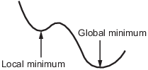
A local minimum of a function is a point where the function value is smaller than at nearby points, but possibly greater than at a distant point.
A global minimum is a point where the function value is smaller than at all other feasible points.
Optimization Toolbox™ solvers typically find a local minimum. (This local minimum can be a global minimum.) They find the minimum in the basin of attraction of the starting point. For more information about basins of attraction, see Basins of Attraction.
The following are exceptions to this general rule.
Linear programming problems and positive definite quadratic programming problems are convex, with convex feasible regions, so they have only one basin of attraction. Depending on the specified options,
linprogignores any user-supplied starting point, andquadprogdoes not require one, even though you can sometimes speed a minimization by supplying a starting point.Global Optimization Toolbox functions, such as
simulannealbnd, attempt to search more than one basin of attraction.
Searching for a Smaller Minimum
If you need a global minimum, you must find an initial value for your solver in the basin of attraction of a global minimum.
You can set initial values to search for a global minimum in these ways:
Use a regular grid of initial points.
Use random points drawn from a uniform distribution if all of the problem coordinates are bounded. Use points drawn from normal, exponential, or other random distributions if some components are unbounded. The less you know about the location of the global minimum, the more spread out your random distribution should be. For example, normal distributions rarely sample more than three standard deviations away from their means, but a Cauchy distribution (density 1/(π(1 + x2))) makes greatly disparate samples.
Use identical initial points with added random perturbations on each coordinate—bounded, normal, exponential, or other.
If you have a Global Optimization Toolbox license, use the
GlobalSearch(Global Optimization Toolbox) orMultiStart(Global Optimization Toolbox) solvers. These solvers automatically generate random start points within bounds.To search using a variety of initial conditions and solvers automatically, run Optimization Explorer on your problem.
The more you know about possible initial points, the more focused and successful your search will be.
Basins of Attraction
If an objective function f(x) is smooth, the vector –∇f(x) points in the direction where f(x) decreases most quickly. The equation of steepest descent, namely
yields a path x(t) that goes to a local minimum as t increases. Generally, initial values x(0) that are near each other give steepest descent paths that tend towards the same minimum point. The basin of attraction for steepest descent is the set of initial values that lead to the same local minimum.
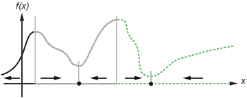
This figure shows two one-dimensional minima. The figure shows different basins of attraction with different line styles, and indicates the directions of steepest descent with arrows. For this and subsequent figures, black dots represent local minima. Every steepest descent path, starting at a point x(0), goes to the black dot in the basin containing x(0).
One-dimensional basins
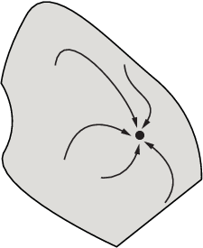
This figure shows how steepest descent paths can be more complicated in more dimensions.
One basin of attraction, showing steepest descent paths from various starting points
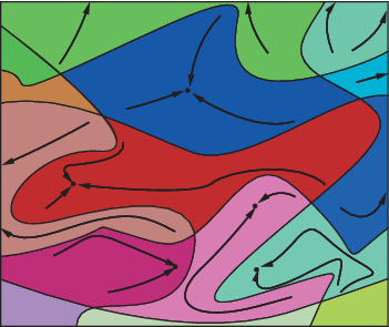
This figure shows even more complicated paths and basins of attraction.
Several basins of attraction
Constraints can break up one basin of attraction into several pieces. For example, consider minimizing y subject to:
y ≥ |x|
y ≥ 5 – 4(x–2)2.
This figure shows the two basins of attraction with the final points.
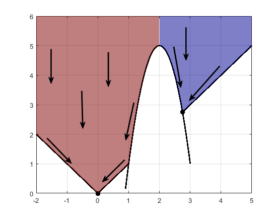
![]() Code for Generating the Figure
Code for Generating the Figure
The steepest descent paths are straight lines down to the constraint boundaries. From the constraint boundaries, the steepest descent paths travel down along the boundaries. The final point is either (0,0) or (11/4,11/4), depending on whether the initial x-value is above or below 2.