使用线性规划实现长期投资最大化：基于求解器

打开实时脚本

此示例显示如何使用 Optimization Toolbox ® 中的 linprog 求解器来求解固定年限内具有确定性回报的投资问题 T。问题在于如何将您的资金分配到可用的投资中，以最大化您的最终财富。此示例使用基于求解器的方法。

问题表示

假设您有初始金额 Capital_0，准备在 T 年期限内投资 N 零息债券。每张债券每年支付复利，并在到期时支付本金和复利。目标是使 T 年后的总金额最大化。

您可以添加一个约束，即任何单项投资都不能超过您总资本的一定比例。

这个示例首先展示了小案例的问题设置，然后构造了一般情况。

您可以将其建模为线性规划问题。因此，为了优化您的财富，请将该问题构造为可以使用 linprog 求解器求解的问题。

介绍性示例

从一个小示例开始：

Capital_0 的投资起始金额为 1000 美元。
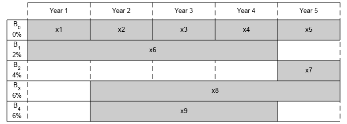
时间段 T 为 5 年。
N 债券的数量为 4。
为了模拟未投资资金，每年提供一个期权 B0，其到期期限为 1 年，利率为 0%。
债券 1，记为 B1，可在第 1 年购买，期限为 4 年，利率为 2%。
债券 2，标记为 B2，可在第 5 年购买，期限为 1 年，利率为 4%。
债券 3，标记为 B3，可在第 2 年购买，期限为 4 年，利率为 6%。
债券 4，标记为 B4，可在第 2 年购买，期限为 3 年，利率为 6%。

通过将第一个期权 B0 拆分为 5 张债券，期限为 1 年，利率为 0%，该问题可以等效建模为总共有 9 张可用债券，因此对于 k=1..9

向量 PurchaseYears 的条目 k 代表债券 k 可购买的年份。
向量 Maturity 的条目 k 代表债券 k 的到期期限 $m_{k}$ 。
向量 InterestRates 的条目 k 代表债券 k 的利率 $ρ_{k}$ 。

通过代表每张债券可用购买时间和期限的水平条来直观地展示这个问题。

% Time period in years
T = 5;
% Number of bonds
N = 4;
% Initial amount of money
Capital_0 = 1000;
% Total number of buying opportunities
nPtotal = N+T;
% Purchase times
PurchaseYears = [1;2;3;4;5;1;5;2;2];
% Bond durations
Maturity = [1;1;1;1;1;4;1;4;3];
% Interest rates
InterestRates = [0;0;0;0;0;2;4;6;6];

plotInvestments(N,PurchaseYears,Maturity,InterestRates)

决策变量

用向量 x 表示您的决策变量，其中 x(k) 是债券 k 的投资美元金额，对于 k=1..9。到期后，投资 x(k) 的收益为

$x (k) (1 + ρ_{k} / 100)^{m_{k}} .$

定义 $β_{k} = 1 + ρ_{k} / 100$ 并将 $r_{k}$ 定义为债券 k 的总回报：

$r_{k} = (1 + ρ_{k} / 100)^{m_{k}} = β_{k}^{m_{k}} .$

% Total returns
finalReturns = (1+InterestRates/100).^Maturity;

目标函数

目标是选择投资来最大化年末所收集的资金量 T。从图中可以看出，投资是在各个中间年份收集并再投资的。在第 T 年末，您可以收回投资 5、7 和 8 所返还的资金，这代表了您的最终财富：

$\max_{x} x_{5} r_{5} + x_{7} r_{7} + x_{8} r_{8}$

为了将此问题转化为 linprog 求解的形式，请使用 x(j) 系数的负数将此最大化问题转化为最小化问题：

$\min_{x} f^{T} x$

替换为：

$f = [0; 0; 0; 0; - r_{5}; 0; - r_{7}; - r_{8}; 0]$

f = zeros(nPtotal,1);
f([5,7,8]) = [-finalReturns(5),-finalReturns(7),-finalReturns(8)];

线性约束：不要投资超过您拥有的

每年，您都会有一定数量的资金可用于购买债券。从第 1 年开始，您可以将初始资本投资于购买期权 $x_{1}$ 和 $x_{6}$ ，因此：

$x_{1} + x_{6} = {C a p i t a l}_{0}$

然后在接下来的几年里，您收集到期债券的收益，并将其再投资于新的可用债券以获得方程组：

$\begin{array}{ll} x_{2} + x_{8} + x_{9} & = r_{1} x_{1} \\ x_{3} & = r_{2} x_{2} \\ x_{4} & = r_{3} x_{3} \\ x_{5} + x_{7} & = r_{4} x_{4} + r_{6} x_{6} + r_{9} x_{9} \end{array}$

将这些方程写成 $A e q x = b e q$ 的形式，其中 $A e q$ 矩阵的每一行对应于当年需要满足的等式：

$A e q = [\begin{array}{ccccccccc} 1 & 0 & 0 & 0 & 0 & 1 & 0 & 0 & 0 \\ - r_{1} & 1 & 0 & 0 & 0 & 0 & 0 & 1 & 1 \\ 0 & - r_{2} & 1 & 0 & 0 & 0 & 0 & 0 & 0 \\ 0 & 0 & - r_{3} & 1 & 0 & 0 & 0 & 0 & 0 \\ 0 & 0 & 0 & - r_{4} & 1 & - r_{6} & 1 & 0 & - r_{9} \end{array}]$

$b e q = [\begin{array}{c} {C a p i t a l}_{0} \\ 0 \\ 0 \\ 0 \end{array}]$

Aeq = spalloc(N+1,nPtotal,15);
Aeq(1,[1,6]) = 1;
Aeq(2,[1,2,8,9]) = [-1,1,1,1];
Aeq(3,[2,3]) = [-1,1];
Aeq(4,[3,4]) = [-1,1];
Aeq(5,[4:7,9]) = [-finalReturns(4),1,-finalReturns(6),1,-finalReturns(9)];

beq = zeros(T,1);
beq(1) = Capital_0;

边界约束：禁止借贷

因为每个投资金额必须为正，所以解向量 $x$ 中的每个条目都必须为正。通过在解向量 $x$ 上设置下界 lb 来包含此约束。解向量没有明确的上界。因此，将上界 ub 设置为空。

lb = zeros(size(f));
ub = [];

求解问题

求解这个问题时，对您可以投资债券的金额没有任何约束。内点算法可以用来求解此类线性规划问题。

options = optimoptions('linprog','Algorithm','interior-point');
[xsol,fval,exitflag] = linprog(f,[],[],Aeq,beq,lb,ub,options);

Solution found during presolve.

可视化解

退出标志为 1，表示求解器找到了解。作为第二个 linprog 输出参量返回的值 -fval 对应于最终财富。绘制一段时间内您的投资图表。

fprintf('After %d years, the return for the initial $%g is $%g \n',...
    T,Capital_0,-fval);

After 5 years, the return for the initial $1000 is $1262.48

plotInvestments(N,PurchaseYears,Maturity,InterestRates,xsol)

有限持股的最优投资

为了分散您的投资，您可以选择将投资于任何一只债券的金额限制为当年总资本的一定百分比 Pmax（包括目前处于到期期的债券的回报）。您将获得以下不等式系统：

$\begin{array}{ll} x_{1} & \leq P m a x \times {C a p i t a l}_{0} \\ x_{2} & \leq P m a x \times (β_{1} x_{1} + β_{6} x_{6}) \\ x_{3} & \leq P m a x \times (β_{2} x_{2} + β_{6}^{2} x_{6} + β_{8} x_{8} + β_{9} x_{9}) \\ x_{4} & \leq P m a x \times (β_{3} x_{3} + β_{6}^{3} x_{6} + β_{8}^{2} x_{8} + β_{9}^{2} x_{9}) \\ x_{5} & \leq P m a x \times (β_{4} x_{4} + β_{6}^{4} x_{4} + β_{8}^{3} x_{8} + β_{9}^{3} x_{9}) \\ x_{6} & \leq P m a x \times {C a p i t a l}_{0} \\ x_{7} & \leq P m a x \times (β_{4} x_{4} + β_{6}^{4} x_{4} + β_{8}^{3} x_{8} + β_{9}^{3} x_{9}) \\ x_{8} & \leq P m a x \times (β_{1} x_{1} + β_{6} x_{6}) \\ x_{9} & \leq P m a x \times (β_{1} x_{1} + β_{6} x_{6}) \end{array}$

将这些不等式以矩阵形式 Ax <= b 表示。

为了建立不等式系统，首先生成一个矩阵 yearlyReturns，其中包含第 j 年第 i 行第 j 列中以 i 为索引的债券的收益。将该系统表示为稀疏矩阵。

% Maximum percentage to invest in any bond
Pmax = 0.6;

% Build the return for each bond over the maturity period as a sparse
% matrix
cumMaturity = [0;cumsum(Maturity)];
xr = zeros(cumMaturity(end-1),1);
yr = zeros(cumMaturity(end-1),1);
cr = zeros(cumMaturity(end-1),1);
for i = 1:nPtotal
    mi = Maturity(i); % maturity of bond i
    pi = PurchaseYears(i); % purchase year of bond i
    idx = cumMaturity(i)+1:cumMaturity(i+1); % index into xr, yr and cr
    xr(idx) = i; % bond index
    yr(idx) = pi+1:pi+mi; % maturing years
    cr(idx) = (1+InterestRates(i)/100).^(1:mi); % returns over the maturity period
end
yearlyReturns = sparse(xr,yr,cr,nPtotal,T+1);

% Build the system of inequality constraints
A = -Pmax*yearlyReturns(:,PurchaseYears)'+ speye(nPtotal);

% Left-hand side
b = zeros(nPtotal,1);
b(PurchaseYears == 1) = Pmax*Capital_0;

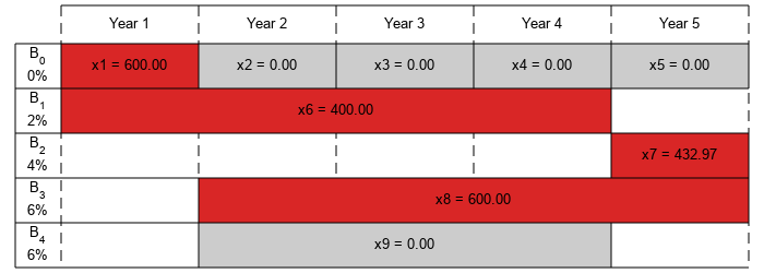
通过对任何一项资产的投资不超过 60% 来求解问题。绘制购买结果图。请注意，您的最终财富将少于没有此约束的投资。

[xsol,fval,exitflag] = linprog(f,A,b,Aeq,beq,lb,ub,options);

Minimum found that satisfies the constraints.

Optimization completed because the objective function is non-decreasing in feasible directions, to within the function tolerance, and constraints are satisfied to within the constraint tolerance.

fprintf('After %d years, the return for the initial $%g is $%g \n',...
    T,Capital_0,-fval);

After 5 years, the return for the initial $1000 is $1207.78

plotInvestments(N,PurchaseYears,Maturity,InterestRates,xsol)

任意尺寸模型

为该问题的一般版本创建一个模型。使用 T = 30 年和 400 个随机生成的债券（利率从 1% 到 6%）来说明。此设置产生一个具有 430 个决策变量的线性规划问题。等式约束系统由维度为 30×430 的稀疏矩阵 Aeq 表示，不等式约束系统由维度为 430×430 的稀疏矩阵 A 表示。

% for reproducibility
rng default 
% Initial amount of money
Capital_0 = 1000;
% Time period in years
T = 30;
% Number of bonds
N = 400;
% Total number of buying opportunities
nPtotal = N+T;
% Generate random maturity durations
Maturity = randi([1 T-1],nPtotal,1);
% Bond 1 has a maturity period of 1 year
Maturity(1:T) = 1;
% Generate random yearly interest rate for each bond
InterestRates = randi(6,nPtotal,1);
% Bond 1 has an interest rate of 0 (not invested)
InterestRates(1:T) = 0;
% Compute the return at the end of the maturity period for each bond:
finalReturns = (1+InterestRates/100).^Maturity;

% Generate random purchase years for each option
PurchaseYears = zeros(nPtotal,1);
% Bond 1 is available for purchase every year
PurchaseYears(1:T)=1:T;
for i=1:N
    % Generate a random year for the bond to mature before the end of
    % the T year period
    PurchaseYears(i+T) = randi([1 T-Maturity(i+T)+1]);
end

% Compute the years where each bond reaches maturity
SaleYears = PurchaseYears + Maturity;

% Initialize f to 0
f = zeros(nPtotal,1);
% Indices of the sale opportunities at the end of year T
SalesTidx = SaleYears==T+1;
% Expected return for the sale opportunities at the end of year T
ReturnsT = finalReturns(SalesTidx);
% Objective function
f(SalesTidx) = -ReturnsT;


% Generate the system of equality constraints.
% For each purchase option, put a coefficient of 1 in the row corresponding
% to the year for the purchase option and the column corresponding to the
% index of the purchase oportunity
xeq1 = PurchaseYears;
yeq1 = (1:nPtotal)';
ceq1 = ones(nPtotal,1);

% For each sale option, put -\rho_k, where \rho_k is the interest rate for the
% associated bond that is being sold, in the row corresponding to the
% year for the sale option and the column corresponding to the purchase
% oportunity
xeq2 = SaleYears(~SalesTidx);
yeq2 = find(~SalesTidx);
ceq2 = -finalReturns(~SalesTidx);

% Generate the sparse equality matrix
Aeq = sparse([xeq1; xeq2], [yeq1; yeq2], [ceq1; ceq2], T, nPtotal);

% Generate the right-hand side
beq = zeros(T,1);
beq(1) = Capital_0;

% Build the system of inequality constraints
% Maximum percentage to invest in any bond
Pmax = 0.4;

% Build the returns for each bond over the maturity period
cumMaturity = [0;cumsum(Maturity)];
xr = zeros(cumMaturity(end-1),1);
yr = zeros(cumMaturity(end-1),1);
cr = zeros(cumMaturity(end-1),1);
for i = 1:nPtotal
    mi = Maturity(i); % maturity of bond i
    pi = PurchaseYears(i); % purchase year of bond i
    idx = cumMaturity(i)+1:cumMaturity(i+1); % index into xr, yr and cr
    xr(idx) = i; % bond index
    yr(idx) = pi+1:pi+mi; % maturing years
    cr(idx) = (1+InterestRates(i)/100).^(1:mi); % returns over the maturity period
end
yearlyReturns = sparse(xr,yr,cr,nPtotal,T+1);

% Build the system of inequality constraints
A = -Pmax*yearlyReturns(:,PurchaseYears)'+ speye(nPtotal);

% Left-hand side
b = zeros(nPtotal,1);
b(PurchaseYears==1) = Pmax*Capital_0;

% Add the lower-bound constraints to the problem.
lb = zeros(nPtotal,1);

无限持股解

首先，利用内点算法求解无不等式约束的线性规划问题。

% Solve the problem without inequality constraints
options = optimoptions('linprog','Algorithm','interior-point');
tic
[xsol,fval,exitflag] = linprog(f,[],[],Aeq,beq,lb,[],options);

Minimum found that satisfies the constraints.

Optimization completed because the objective function is non-decreasing in feasible directions, to within the function tolerance, and constraints are satisfied to within the constraint tolerance.

toc

Elapsed time is 0.022026 seconds.

fprintf('\nAfter %d years, the return for the initial $%g is $%g \n',...
    T,Capital_0,-fval);

After 30 years, the return for the initial $1000 is $5167.58

有限持股解

现在，求解不等式约束的问题。

% Solve the problem with inequality constraints
options = optimoptions('linprog','Algorithm','interior-point');
tic
[xsol,fval,exitflag] = linprog(f,A,b,Aeq,beq,lb,[],options);

Minimum found that satisfies the constraints.

Optimization completed because the objective function is non-decreasing in feasible directions, to within the function tolerance, and constraints are satisfied to within the constraint tolerance.

toc

Elapsed time is 1.908206 seconds.

fprintf('\nAfter %d years, the return for the initial $%g is $%g \n',...
    T,Capital_0,-fval);

After 30 years, the return for the initial $1000 is $5095.26

尽管约束的数量增加了 10 个数量级，求解器找到解的时间却增加了 100 个数量级。这种性能差异部分是由矩阵 A 所示的不等式系统中的密集列引起的。这些列对应于期限较长的债券，如下图所示。

% Number of nonzero elements per column
nnzCol = sum(spones(A));

% Plot the maturity length vs. the number of nonzero elements for each bond
figure;
plot(Maturity,nnzCol,'o');
xlabel('Maturity period of bond k')
ylabel('Number of nonzero in column k of A')

约束中的密集列导致求解器内部矩阵中的密集块，从而导致其稀疏方法的效率损失。为了加快求解器的速度，请尝试对列密度不太敏感的对偶单纯形算法。

% Solve the problem with inequality constraints using dual simplex
options = optimoptions('linprog','Algorithm','dual-simplex');
tic
[xsol,fval,exitflag] = linprog(f,A,b,Aeq,beq,lb,[],options);

Optimal solution found.

toc

Elapsed time is 0.088663 seconds.

fprintf('\nAfter %d years, the return for the initial $%g is $%g \n',...
    T,Capital_0,-fval);

After 30 years, the return for the initial $1000 is $5095.26

在这种情况下，对偶单纯形算法花费更少的时间来获得相同的解。

定性结果分析

为了了解 linprog 找到的解，请将其与 fmax 进行比较，如果您可以在整个 30 年期间将所有启动资金投资于一张利率为 6%（最高利率）的债券，您将获得该金额。您还可以计算与您的最终财富相对应的等值利率。

% Maximum amount
fmax = Capital_0*(1+6/100)^T;
% Ratio (in percent)
rat = -fval/fmax*100;
% Equivalent interest rate (in percent)
rsol = ((-fval/Capital_0)^(1/T)-1)*100;

fprintf(['The amount collected is %g%% of the maximum amount $%g '...
    'that you would obtain from investing in one bond.\n'...
    'Your final wealth corresponds to a %g%% interest rate over the %d year '...
    'period.\n'], rat, fmax, rsol, T)

The amount collected is 88.7137% of the maximum amount $5743.49 that you would obtain from investing in one bond.
Your final wealth corresponds to a 5.57771% interest rate over the 30 year period.

plotInvestments(N,PurchaseYears,Maturity,InterestRates,xsol,false)