用于并行并发工作流中高效资源管理的分区池
此示例展示了如何使用池分区来有效管理和优化并行工作流中的资源分配。
并行池分区允许您同时执行多个工作流,而不会相互干扰,从而实现对每个工作流资源使用的精确控制。通过将特定计算任务(如 parfor、parfeval 和 spmd)分配给指定的池分区,您可以确保每个工作流独立且高效地运行。
这种方法对于组织并行管道工作流特别有利,因为不同阶段可能需要不同的资源。在这种情况下,池分区通过定制资源分配以满足每个阶段的要求,促进数据在管道中的顺畅流动。此外,在同时运行多个独立的工作流时,池分区非常有用,因为它们有助于管理和限制每个工作流消耗的资源。
此示例说明了在执行并行仿真管道时,如何使用池分区与多个 GPU 以及蒙特卡罗路径规划仿真一起使用。您可以调整此方法来同时管理各种工作流的执行,以确保最佳的资源分配和工作流性能。
创建并行池分区
启动一个具有 16 个工作单元的并行池。在此示例中,myCluster 配置文件从远程集群请求一个具有 16 个工作单元的并行池,其中每个主机有 8 个工作单元和 2 个 GPU。
pool = parpool("myCluster",16);Starting parallel pool (parpool) using the 'myCluster' profile ... Connected to parallel pool with 16 workers.
使用分区函数创建符合仿真管道不同阶段要求的池分区。
使用 partition 函数创建一个池分区,为每个可用 GPU 配置一个工作单元,以获得最佳性能。如果池中没有 GPU,则 gpuPool 分区返回一个空的 parallel.pool 对象,GPU 计算在客户端上运行。
[gpuPool,cpuPool] = partition(pool,"MaxNumWorkersPerGPU",1);使用 cpuPool 分区中的剩余工作单元,创建两个额外的分区。一个包含四个工作单元,另一个包含其余工作单元,位于 cpuPool 分区。您需要至少五个工作单元才能并行运行仿真管道和 parfor 循环。如果工作单元不够,请减少 cpuLidarPool 分区的工作单元数。
cpuWorkers = cpuPool.Workers;
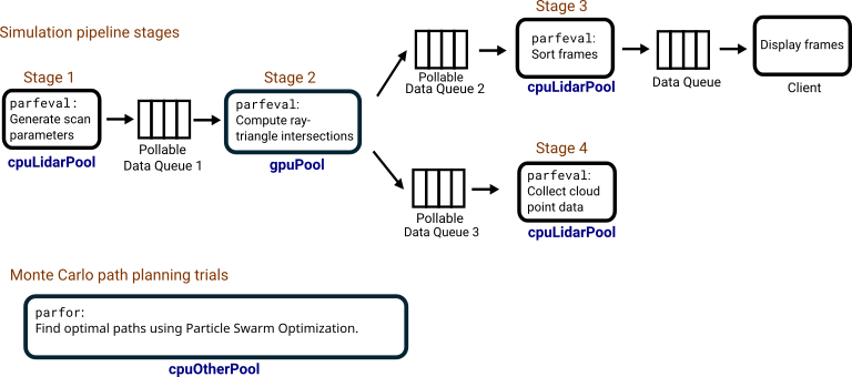
[cpuLidarPool,cpuOtherPool] = partition(cpuPool,"Workers",cpuWorkers(1:4));该图说明了仿真管道阶段和蒙特卡罗路径规划试验如何使用池分区。
在池分区上执行仿真管道
在此示例中,并行仿真管道使用光线追踪对激光雷达扫描系统进行建模。激光雷达传感器与雷达和声纳类似,通过发射激光脉冲,利用其反射回来的信号来测量距离,从而感知周围环境的结构。通过实施光线追踪算法并在多个 GPU 上执行交点计算,您可以仿真激光雷达扫描系统,以收集场景中附近结构的信息,并生成环境的点云地图。
管道计算三角化场景与激光射线之间的交点,以确定有多少光照射到物体表面。为了加快这些计算速度,使用经过修改的 Möller-Trumbore[1] 算法,使其能在 GPU 上运行,并采用 arrayfun 格式。
为了进一步提高仿真速度,将仿真阶段作为并行管道执行,进行多次 parfeval 计算。为了确保不同阶段在正确的工作单元上运行,请在 parfeval 和 gpuPool 分区上运行 cpuLidarPool 计算。
第一阶段:在长期运行的
parfeval计算中,来自cpuLidarPool分区的 CPU 工作单元为每个时间步生成输入参数,例如激光雷达传感器位置和光线方向。工作单元使用可轮询数据队列将这些参数发送到管道的第 2 阶段。该工作单元还会触发一个parfeval计算,在 GPU 上执行光线与三角形相交计算。第二阶段:使用多个
parfeval计算代替一个长时间运行的计算。来自gpuPool分区的 GPU 工作单元运行一个parfeval计算,该计算从可轮询数据队列中轮询来自阶段 1 的数据,找到光线与对象表面的交点,并使用两个可轮询数据队列将结果发送给阶段 3 和 4。第三阶段:一个长时间运行的
parfeval计算对第 2 阶段的结果进行排序,并使用数据队列将它们按顺序发送给客户端进行显示。第四阶段:两个长期运行的
parfeval计算通过聚合第二阶段的交点距离结果生成激光雷达点云。
初始化仿真环境和参数
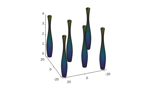
首先,设置一个由多个三角面对象组成的场景。使用在本示例末尾定义的 initializeParameters 函数,指定初始光线位置和运动参数。
params = initializeParameters;
接下来,使用 plotScene 函数可视化场景,该函数在本示例末尾已定义。
plotScene(params);
view([-110.88 31.50])
准备数据队列并定义回调函数
为了在仿真过程中方便不同工作单元之间的数据传输,请混合使用 PollableDataQueue 和 DataQueue 对象。
创建两个 PollableDataQueue 对象,将 Destination 设置为 "any",用于仿真管道。管道中的第一个工作单元为每次扫描生成输入参数,并将参数发送到可轮询数据队列 stage2InputQueue 进行处理。然后,GPU 工作单元之一计算光线与三角形的交点,并将结果发送到可轮询数据队列 stage3SortQueue 和 stage4CloudQueue 以进行进一步处理。
stage2InputQueue = parallel.pool.PollableDataQueue(Destination="any"); % Pollable data queue 1
stage3SortQueue = parallel.pool.PollableDataQueue(Destination="any");  % Pollable data queue 2
stage4CloudQueue = parallel.pool.PollableDataQueue(Destination="any");  % Pollable data queue 3
在此示例中,您在 parfeval 分区上运行多个短暂的 gpuPool 计算,以计算每次扫描的交集。这样,如果有一个工作单元空闲,您就可以在同一个 gpuPool 分区上交错执行其他并行工作。创建一个名为 DataQueue 的 stage2TriggerQueue 对象,并使用 afterEach 函数定义一个函数,在 stage2TriggerQueue 数据队列对象每次接收数据时运行。
当输入参数准备就绪时,运行阶段 1 的工作单元向 stage2TriggerQueue 发送一条消息。在 stage2TriggerQueue 接收到数据后,它会自动提交一个 parfeval 计算任务,以在 findIntersections 分区上执行 gpuPool 函数。请注意,输入数据已位于 stage2InputQueue 可轮询数据队列中。findIntersections 函数在示例末尾定义。
stage2TriggerQueue = parallel.pool.DataQueue;
afterEach(stage2TriggerQueue,@(call) ...
parfeval(gpuPool,@findIntersections,0,stage2InputQueue,stage3SortQueue,stage4CloudQueue));准备并初始化绘图,以可视化来自工作单元的中间扫描数据。prepareScanningPlot 函数在此示例的末尾定义。
[fig,s,rays] = prepareScanningPlot(params);
要跟踪客户端上的扫描进度,请创建一个名为 DataQueue 的 displayQueue 对象。当工作单元将数据发送到 afterEach 数据队列对象时,使用 displayScanFrames 函数运行 displayQueue 函数。displayScanFrames 函数在此示例的末尾定义。
displayQueue = parallel.pool.DataQueue;
afterEach(displayQueue,@(data) displayScanFrames(data,s,rays));
开始仿真管道
第一阶段和第二阶段
对于管道的第一阶段,使用来自 cpuLidarPool 分区的一个工作单元在后台使用 addParamsToQueue 运行 parfeval 函数。addParamsToQueue 函数为每次扫描连续生成输入参数,并将它们发送到可轮询数据队列对象 stage2InputQueue。它还会向 stage2TriggerQueue 数据队列对象发送消息,以在管道的第 2 阶段对 parfeval 分区触发 gpuPool 计算。
当工作单元生成所有扫描输入参数时,它会关闭 stage2InputQueue,以向下一阶段的工作单元发出信号,表明没有更多数据要发送。addParamsToQueue 函数在此示例的末尾定义。
fgenerate = parfeval(cpuLidarPool,@addParamsToQueue,0,params,stage2InputQueue,stage2TriggerQueue);
第三阶段
使用 cpuLidarPool 分区中的工作单元,在后台使用 sortFrames 运行 parfeval 辅助函数。sortFrames 函数反复轮询 stage3SortQueue 可轮询数据队列以获取新帧数据,为帧建立缓冲区,并使用 displayQueue 数据队列以正确的顺序将它们发送给客户端。当前一个阶段的工作单元关闭 sortFrames 可轮询数据队列时,stage3SortQueue 函数停止执行。sortFrames 函数作为支持文件附加到此示例。
fSort = parfeval(cpuLidarPool,@sortFrames,0,stage3SortQueue,displayQueue);
第四阶段
使用来自 collectCloudPointData 分区的的工作单元运行两个 cpuLidarPool 函数实例,以生成云点数据。collectCloudPointData 函数反复轮询 stage4CloudQueue 可轮询数据队列以获取新的交叉数据,并在前一个阶段的工作单元关闭 stage4CloudQueue 可轮询数据队列时停止执行。collectCloudPointData 函数在此示例的末尾定义。
fCloud(1) = parfeval(cpuLidarPool,@collectCloudPointData,1,stage4CloudQueue);
fCloud(2) = parfeval(cpuLidarPool,@collectCloudPointData,1,stage4CloudQueue);
最后,使图形可见,以显示激光雷达仿真的进度。
fig.Visible = "on";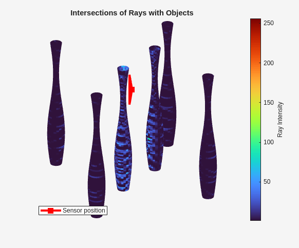
对剩余池分区执行路径规划
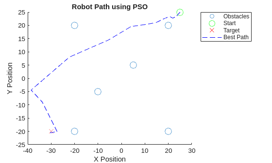
在激光雷达仿真管道运行时,您可以使用剩余的 cpuOtherPool 分区执行其他计算。例如,您可以使用一个 parfor 循环来运行多个路径规划算法的试验,这些算法使用粒子群优化 (PSO)。目标是从起始位置到目标位置找到一条最佳路径,同时避开场景中的物体。
定义环境和 PSO 参数
使用仿真管道中的相同场景设置环境参数,包括起始位置和目标位置。定义对象的半径。
startPos = [25 25];
targetPos = [-30 -20];
objectRadius = ones(size(params.objectPositions,1),1)*2;
obstacles = [params.objectPositions objectRadius];
配置 PSO 算法的参数,例如粒子数、迭代次数和尝试次数。将问题限制在二维空间内。
numParticles = 1000;
numIterations = 300;
dim = 2;
numTrials = 100;
执行路径规划试验
准备记录每次试验的最佳路径和得分。使用 parfor 函数将试验并行化,以提高效率。要在 parfor 分区上运行 cpuOtherPool 循环,请将池对象指定为 parfor 函数的第二个参量。planPathPSO 辅助函数已作为支持文件附加到此示例中。
parfor(trial = 1:numTrials,cpuOtherPool)
[bestPath(trial,:,:),scores(trial)] = planPathPSO(startPos,targetPos, ...
    obstacles,numParticles,dim,numIterations);
end
识别出得分最低的试验,该试验对应于 PSO 算法找到的最佳路径。
[~,bestInd] = min(scores);
在图表上可视化环境、障碍物以及最佳路径。plotBestPath 函数在示例末尾定义。
plotBestPath(obstacles,startPos,bestPath(bestInd,:,:),targetPos);
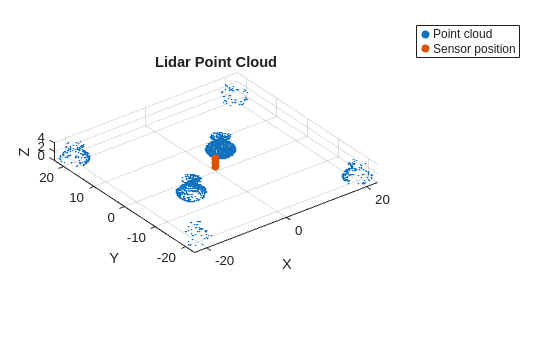
从激光雷达仿真中可视化点云
随着激光雷达仿真管道的完成,您可以从 fCloud parfeval 计算中检索结果。
pointCloud = fetchOutputs(fCloud);
使用在示例末尾定义的 plotPointCloud 函数,可可视化聚合的激光雷达传感器点云检测结果。点云可视化显示了场景中对象的轮廓。
plotPointCloud(pointCloud,params);
参考资料
[1] Möller, Tomas, and Ben Trumbore."Fast, Minimum Storage Ray-Triangle Intersection."Journal of Graphics Tools 2, no. 1 (January 1997):21–28. https://doi.org/10.1080/10867651.1997.10487468.
本地支持函数
addParamsToQueue - 仿真管道第一阶段
addParamsToQueue 函数为每次扫描生成输入参数,并管理将其添加到数据队列中进行处理。对于每一步,它计算光源在物体表面移动时的光源原点,分配一个扫描编号,并将这些数据发送到可轮询数据队列 stage2InputQueue。它还通过向 parfeval 可轮询数据队列发送消息,向 GPU 池发出调度 stage2TriggerQueue 计算的信号。该函数包括队列管理,当队列长度超过指定阈值时,通过暂停来防止输入队列过载。在为所有扫描生成参数后,它关闭 stage2InputQueue 并向 stage2TriggerQueue 提交最终任务以关闭阶段 2 可轮询数据队列。getScanParam 辅助函数作为支持文件附在此示例中。
function addParamsToQueue(params,stage2InputQueue,stage2TriggerQueue)
fN = 0;

numScans = size(params.lidarOrigins,1);

for scan = 1:numScans
    % Set lidar origin (position)
    lidarOrigin = params.lidarOrigins(scan,:);

    for t = 1:params.totalTimeSteps
        data = getScanParam(params,t,lidarOrigin);
        fN = fN + 1;

        % Send scan number and input data to the data queue
        data.fN = fN;
        send(stage2InputQueue,data);

        % Submit parfeval computation on the GPU pool
        send(stage2TriggerQueue,"findIntersections");

        pause(0.5); % Pause to improve visualization

        % Perform some queue management to reduce strain on queue
        while stage2InputQueue.QueueLength > 10
            pause(1);
        end
    end
end

% Close queue after generating all input parameters
close(stage2InputQueue);

% Submit parfeval computation to close stage 2 queues
send(stage2TriggerQueue,"findIntersections");
end
findIntersections - 仿真管道第二阶段
findIntersections 函数处理来自队列的输入参数,使用 GPU 加速计算光线与 3D 对象三角形之间的交点。它从可轮询数据队列 stage2InputQueue 中检索数据,将光线源和方向转换为 gpuArray 对象,并使用 arrayfun 在 GPU 上执行光线与三角形相交计算。它收集结果,提取第一个交点,并使用命中次数更新数据结构。最后,它将扫描编号、更新后的数据和交叉点分别发送到可轮询数据队列 stage3SortQueue 和 stage4CloudQueue。rayTriangleIntersection 辅助函数已作为支持文件附加到此示例中。当 stage2InputQueue 中没有可用数据,且 poll 将 OK 返回为 false(因为 stage2InputQueue 的可轮询数据队列已关闭)时,该函数关闭 stage3SortQueue 和 stage4CloudQueue 以指示处理结束。
function findIntersections(stage2InputQueue,stage3SortQueue,stage4CloudQueue)
[data,OK] = poll(stage2InputQueue,inf);
if OK
    rayOriginsGPU = gpuArray(data.lidarOrigin);
    rayDirectionsGPU = gpuArray(data.rayDirections);

    % Convert to gpuArray and calculate ray triangle intersections on the GPU
    [Hits,intXs,intYs,intZs,intersectionDistances] = arrayfun(@rayTriangleIntersection, ...
        rayOriginsGPU(:,1),rayOriginsGPU(:,2),rayOriginsGPU(:,3), ...
        rayDirectionsGPU(:,1),rayDirectionsGPU(:,2),rayDirectionsGPU(:,3), ...
        data.A(:,1)',data.B(:,1)',data.C(:,1)',...
        data.A(:,2)',data.B(:,2)',data.C(:,2)', ...
        data.A(:,3)',data.B(:,3)',data.C(:,3)');

    data.rayDirections = [];

    % Find the closest intersection for each ray
    [~,minIndices] = min(abs(intersectionDistances),[],2,"omitnan");

    % Extract the first intersection points using the indices
    numRays = size(intXs,1);
    X = intXs(sub2ind(size(intXs),(1:numRays)',minIndices));
    Y = intYs(sub2ind(size(intYs),(1:numRays)',minIndices));
    Z = intZs(sub2ind(size(intZs),(1:numRays)',minIndices));

    % Add intersection values to data structure
    data.numHits = gather(sum(Hits,1));

    % Send scan number and scan data to next worker to sort for display
    output{1} = data.fN;
    output{2} = data;
    send(stage3SortQueue,output);

    % Send intersection points to next worker
    cloudData.intXs = gather(X);
    cloudData.intYs = gather(Y);
    cloudData.intZs = gather(Z);
    send(stage4CloudQueue,cloudData);

elseif ~OK
    close(stage3SortQueue);
    close(stage4CloudQueue);
end
end
collectCloudPointData - 仿真管道第四阶段
collectCloudPointData 函数处理光线交点计算生成的数据,以收集并精化三维交点。它会持续轮询一个队列以获取新数据,过滤掉无效条目,对数据进行降采样,并将坐标四舍五入到指定精度。当 stage4CloudQueue 中没有数据,且 poll 返回 OK 作为 false(因为前一个阶段的工作单元关闭了 stage4CloudQueue 可轮询数据队列),函数停止执行并返回点云数据。
function pointCloud = collectCloudPointData(stage4CloudQueue)
intersectionPoints = [];
OK = true;
while OK
    [cloudData,OK] = poll(stage4CloudQueue,inf);
    if ~isempty(cloudData)
        % Flatten the matrices
        X_flat = cloudData.intXs(:);
        Y_flat = cloudData.intYs(:);
        Z_flat = cloudData.intZs(:);

        % Create a logical mask for valid intersections
        validMask = ~isnan(X_flat);

        % Filter the points using the valid mask
        validX = X_flat(validMask);
        validY = Y_flat(validMask);
        validZ = Z_flat(validMask);

        % Combine the valid points into a single matrix
        thisIntersectionPoints = [validX validY validZ];
        % Downsample by selecting every nth point
        n = 5; % Downsample factor
        thisIntersectionPoints = thisIntersectionPoints(1:n:end,:);

        % Round coordinates to reduce precision
        precisionFactor = 0.01;
        thisIntersectionPoints = round(thisIntersectionPoints/precisionFactor)*precisionFactor;

        intersectionPoints = [intersectionPoints;thisIntersectionPoints];
        pointCloud = intersectionPoints;

    elseif ~OK
        pointCloud = intersectionPoints;
        return
    end
end
end
initializeParameters
initializeParameters 函数初始化并返回一个包含激光雷达扫描系统仿真参数的结构。它设置每转的射线数、垂直层数、传感器的视场和激光雷达扫描的原点位置。它还定义了场景中对象的表面轮廓,并使用 createTriangulatedSurfaces 辅助函数生成三角化表面数据。createTriangulatedSurfaces 辅助函数已作为支持文件附加到此示例中。
function params = initializeParameters
% Define the object and create the triangulated surface
params.surfProfile = 80;
params.objectPositions = [-20 -20;20 -20;-20 20;20 20;-10 -5;5 5];
[params.A,params.B,params.C,params.indices] = createTriangulatedSurfaces(params.surfProfile, ...
    params.objectPositions);

% LiDAR Parameters
params.numRaysPerRevolution = 1000; % Number of rays in one complete horizontal revolution
params.numLayers = 40; % Number of vertical layers
params.verticalFOV = 60; % Vertical field of view in degrees

% Simulation Parameters
params.angularSpeed = 10; % Degrees per time step
params.totalTimeSteps = 36;
params.lidarOrigins = single([0,0,1;0,0,2;0,0,3]); % Set lidar origin (position
end
displayScanFrames
displayScanFrames 函数通过根据新数据修改表面图和光源,更新激光雷达扫描数据的可视化效果。
function displayScanFrames(data,s,rays)
s(1).UserData = s(1).UserData + data.numHits;
indices = s(2).UserData;

% Normalize hits to range between 1 and 256
normalizedHits = rescale(s(1).UserData,1,256);

% Update surface plot with new intensities
colors = repmat(normalizedHits',1,3);

for idx = 1:length(indices)
rowStart = indices(idx,1);
rowEnd = indices(idx,2);
s(idx).CData = colors(rowStart:rowEnd,:);
end

% Update origin of light source
for idx = 1:size(data.rayX,1)
rays(idx).XData = data.rayX(idx,:);
rays(idx).YData = data.rayY(idx,:);
rays(idx).ZData = data.rayZ(idx,:);
end
drawnow limitrate nocallbacks;
end
prepareScanningPlot
prepareScanningPlot 函数设置一个图形和轴,以可视化光线与对象的交点。次要坐标轴以红色标记显示光源的位置。
function [fig,s,rays] = prepareScanningPlot(params)
fig = figure(Position=[933 313 582 483],Visible="off");

%  Create axes for surface
colors = zeros(size(params.A));

hold on
for idx = 1:length(params.indices)
rowStart = params.indices(idx,1);
rowEnd = params.indices(idx,2);
s(idx) = surf(params.A(rowStart:rowEnd,:), ...
    params.B(rowStart:rowEnd,:), ...
    params.C(rowStart:rowEnd,:), ...
    colors(rowStart:rowEnd,:), ...
    EdgeColor="none");
end
hold off
view([-110.88 31.50])

title("Intersections of Rays with Objects");
% Add title and axes labels
axis square;
axis off
colormap turbo;
c = colorbar;
c.Label.String = "Ray Intensity";
view(160,28);
s(1).UserData = zeros(1,size(params.A,1));
s(2).UserData = params.indices;

hold on
for idx = 1:3
rays(idx) = plot3([NaN NaN],[NaN NaN],[NaN NaN],"r",LineWidth=3);
end
rays(1).MarkerIndices = 1;
rays(1).Marker = "square";
rays(1).MarkerSize = 8;
rays(1).MarkerFaceColor = "r";
rays(1).DisplayName = "Sensor position";
hold off
axis off
legend(rays(1),Location="southwest")
end
plotScene
plotScene 函数显示激光雷达仿真的场景。
function plotScene(params)
figure;
hold on
for idx = 1:length(params.indices)
    rowStart = params.indices(idx,1);
    rowEnd = params.indices(idx,2);
    surf(params.A(rowStart:rowEnd,:), ...
        params.B(rowStart:rowEnd,:), ...
        params.C(rowStart:rowEnd,:));
end
hold off
view(3)
axis square
end
plotPointCloud
plotPointCloud 函数显示来自激光雷达仿真管道的累积点云数据。
function plotPointCloud(pointCloud,params)
figure;
scatter3(pointCloud(:,1),pointCloud(:,2),pointCloud(:,3),1,"filled");
hold on
scatter3(params.lidarOrigins(:,1),params.lidarOrigins(:,2),params.lidarOrigins(:,3),"filled");
hold off
xlabel("X");
ylabel("Y");
zlabel("Z");
title("Lidar Point Cloud");
legend("Point cloud","Sensor position",Location="bestoutside");
axis equal;
grid on;
end
plotBestPath
plotBestPath 函数显示环境、障碍物以及 PSO 试验中的最佳路径。
function plotBestPath(obstacles,startPos,bestPath,targetPos)
figure;
hold on;
scatter(obstacles(:,1),obstacles(:,2),100);
plot(startPos(1),startPos(2),"go","MarkerSize",10);
plot(targetPos(1),targetPos(2),"rx","MarkerSize",10);
plot(bestPath(1,:,1),bestPath(1,:,2),"b--");
legend("Obstacles","Start","Target","Best Path",Location="bestoutside");
title("Robot Path using PSO");
xlabel("X Position");
ylabel("Y Position");
hold off;
end