Dynamic Analysis of Clamped Beam

Open Live Script

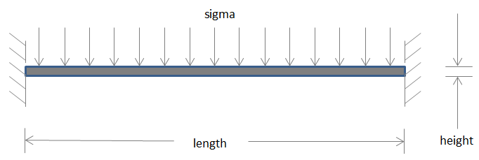
This example shows how to analyze the dynamic behavior of a beam under a uniform pressure load and clamped at both ends.

This example uses the Imperial system of units. If you replace them with values specified in the metric system, ensure that you specify all values using the same system.

In this example, the pressure load is suddenly applied at time equal to zero. The pressure magnitude is high enough to produce deflections on the same order as the beam thickness. Accurate prediction of this type of behavior requires geometrically nonlinear elasticity equations. This example solves the clamped beam elasticity problem using both linear and nonlinear formulations of elasticity equations.

One approach to handling the large deflections is to consider the elasticity equations in the deformed position. However, the toolbox uses the equations based on the original geometry. Therefore, you must use a Lagrangian formulation of nonlinear elasticity where stresses, strains, and coordinates refer to the original geometry. The Lagrangian formulation of the equilibrium equations is

$ρ u_{}^{¨} - \nabla \cdot (F \cdot S) = f$

where $ρ$ is the material density, $u$ is the displacement vector, $F$ is the deformation gradient, $S$ is the second Piola-Kirchoff stress tensor, and $f$ is the body force vector. You also can write this equation in the tensor form:

$ρ {u_{}^{¨}}_{i} - \frac{\partial}{\partial x_{j}} ((\frac{\partial u_{i}}{\partial x_{k}} + δ_{i k}) S_{k j}) = f_{i}$

Although this formulation accounts for large deflections, it assumes that the strains remain small, so that linear elastic constitutive relations apply. For the 2-D plane stress case, you can write the constitutive relations in matrix form:

${\begin{array}{c} S_{11} \\ S_{22} \\ S_{12} \end{array}} = [\begin{array}{ccc} C_{11} & C_{12} \\ C_{12} & C_{22} \\ 2 G_{12} \end{array}] {\begin{array}{c} E_{11} \\ E_{22} \\ E_{12} \end{array}}$

$E_{i j}$ is the Green-Lagrange strain tensor:

$E_{i j} = \frac{1}{2} (\frac{\partial u_{i}}{\partial x_{j}} + \frac{\partial u_{j}}{\partial x_{i}} + \frac{\partial u_{k}}{\partial x_{i}} \frac{\partial u_{k}}{\partial x_{j}})$

For an isotropic material:

$C_{11} = C_{22} = \frac{E}{1 - ν^{2}}$

$C_{12} = \frac{E ν}{1 - ν^{2}}$

$G_{12} = \frac{E}{2 (1 + ν)}$

where $E$ is the Young's modulus, and $ν$ is the Poisson's ratio. For more details about the Lagrangian formulation for nonlinear elasticity, see [1].

These equations completely define the geometrically nonlinear plane stress problem. This example uses Symbolic Math Toolbox™ to define the c coefficient in the form required by Partial Differential Equation Toolbox™. The c coefficient is a function cCoefficientLagrangePlaneStress. You can use it with any geometric nonlinear plane stress analysis of a model made from an isotropic material. You can find it under matlab/R20XXx/examples/pde/main.

Linear Solution

Create a PDE model for a system of two equations.

model = createpde(2);

Create the following beam geometry.

Geometry of a beam under a uniform pressure load and clamped at both ends.

Specify the length and thickness of the beam.

blength = 5; % Beam length, in
height = 0.1; % Thickness of the beam, in

Because the beam geometry and loading are symmetric about the beam center, you can simplify the model by considering only the right half of the beam.

l2 = blength/2;
h2 = height/2;

Create the edges of the rectangle representing the beam.

rect = [3 4 0 l2 l2 0 -h2 -h2  h2 h2]';
g = decsg(rect,'R1',('R1')');

Create the geometry from the edges and include it in the model.

pg = geometryFromEdges(model,g);

Plot the geometry with the edge labels.

figure
pdegplot(g,EdgeLabels="on")
axis([-.1 1.1*l2 -5*h2 5*h2])

Figure contains an axes object. The axes object contains 5 objects of type line, text.

Derive the equation coefficients using the material properties. For the linear case, the c coefficient matrix is constant.

E = 3.0e7; % Young's modulus of the material, lbs/in^2
gnu = 0.3; % Poisson's ratio of the material
rho = 0.3/386; % Density of the material
G = E/(2.*(1 + gnu));
mu = 2*G*gnu/(1 - gnu);
c = [2*G + mu; 0; G;   0; G; mu; 0;  G; 0; 2*G + mu];
f = [0 0]'; % No body forces
specifyCoefficients(model,m=rho,d=0,c=c,a=0,f=f);

Apply the boundary conditions. From the symmetry condition, the x-displacement equals zero at the left edge.

symBC = applyBoundaryCondition(model,"mixed", ...
                               Edge=4,u=0, ...
                               EquationIndex=1);

Because the beam is clamped, the x- and y-displacements equal zero along the right edge.

clampedBC = applyBoundaryCondition(model,"dirichlet",Edge=2,u=[0 0]);

Apply a constant vertical stress along the top edge.

sigma = 2e2;
presBC = applyBoundaryCondition(model,"neumann",Edge=3,g=[0 sigma]);

Set the zero initial displacements and velocities.

setInitialConditions(model,0,0);

Generate a mesh.

generateMesh(model);

Solve the model.

tlist = linspace(0,3e-3,100);
result = solvepde(model,tlist);

Interpolate the solution at the geometry center for the y-component (component 2) at all solution times.

xc = 1.25;
yc = 0;
u4Linear = interpolateSolution(result,xc,yc,2,1:length(tlist));

Nonlinear Solution

Specify the coefficients for the nonlinear case. The cCoefficientLagrangePlaneStress function takes the isotropic material properties and location and state structures, and returns a c-matrix for a nonlinear plane stress analysis. It assumes that strains are small, that is, E and $ν$ are independent of the solution.

c  = @(location,state)cCoefficientLagrangePlaneStress(E,gnu, ...
                                                location,state);
specifyCoefficients(model,m=rho,d=0,c=c,a=0,f=f);

Solve the model.

result = solvepde(model,tlist);

Interpolate the solution at the geometry center for the y-component (component 2) at all solution times.

u4NonLinear = interpolateSolution(result,xc,yc,2,1:length(tlist));

Solution Plots

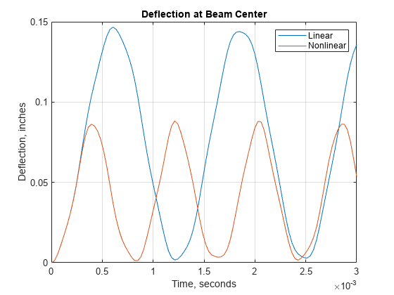
Plot the y-deflection at the center of the beam as a function of time. The nonlinear analysis yields substantially smaller displacements than the linear analysis. This "stress stiffening" effect also results in the higher oscillation frequency from the nonlinear analysis.

figure
plot(tlist,u4Linear(:),tlist,u4NonLinear(:))
legend("Linear","Nonlinear")
title("Deflection at Beam Center")
xlabel("Time, seconds")
ylabel("Deflection, inches")
grid on

Figure contains an axes object. The axes object with title Deflection at Beam Center, xlabel Time, seconds, ylabel Deflection, inches contains 2 objects of type line. These objects represent Linear, Nonlinear.

References

Malvern, Lawrence E. Introduction to the Mechanics of a Continuous Medium. Prentice Hall Series in Engineering of the Physical Sciences. Englewood Cliffs, NJ: Prentice-Hall, 1969.