Eigenvalues and Eigenmodes of Square: PDE Modeler App
This example shows how to compute the eigenvalues and eigenmodes of a square with the corners (-1,-1), (-1,1), (1,1), and (1,-1). This example uses the PDE Modeler app. For programmatic workflow, see Eigenvalues and Eigenmodes of Square.
The eigenvalue PDE problem is . Find the eigenvalues smaller than 10 and the corresponding eigenmodes.
To solve this problem in the PDE Modeler app, follow these steps:
Draw a square with the corners (-1,-1), (-1,1), (1,1), and (1,-1) by using the
pderectfunction.pderect([-1 1 -1 1])
Check that the application mode is set to Generic Scalar.
Specify the boundary conditions. To do this, switch to the boundary mode by selecting Boundary > Boundary Mode. Double-click the boundary to specify the boundary condition.
Specify the Dirichlet condition u = 0 for the left boundary. To do this, specify
h = 1,r = 0.Specify the Neumann condition for the upper and lower boundary. To do this, specify
g = 0,q = 0.Specify the generalized Neumann condition for the right boundary. To do this, specify
g = 0,q = -3/4.
Specify the coefficients by selecting PDE > PDE Specification or clicking the
 button on the toolbar. This is an eigenvalue
problem, so select the Eigenmodes type of PDE. The general
eigenvalue PDE is described by . Thus, for this problem, the coefficients are
button on the toolbar. This is an eigenvalue
problem, so select the Eigenmodes type of PDE. The general
eigenvalue PDE is described by . Thus, for this problem, the coefficients are c = 1,a = 0, andd = 1.Specify the maximum edge size for the mesh by selecting Mesh > Parameters. Set the maximum edge size value to 0.05.
Initialize the mesh by selecting Mesh > Initialize Mesh.
Specify the eigenvalue range by selecting Solve > Parameters. In the resulting dialog box, enter the eigenvalue range as the MATLAB® vector
[-Inf 10].Solve the PDE by selecting Solve > Solve PDE or clicking the
 button on the toolbar. By default, the app plots
the first eigenfunction.
button on the toolbar. By default, the app plots
the first eigenfunction.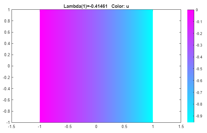
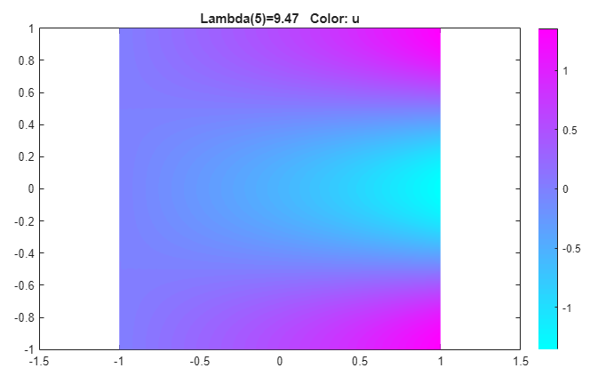
Plot other eigenfunctions by selecting Plot > Parameters and then selecting the corresponding eigenvalue from the drop-down list at the bottom of the dialog box. For example, plot the last eigenfunction in the specified range.
Export the eigenfunctions and eigenvalues to the MATLAB workspace by using the Solve > Export Solution.