interpolateCurrentDensity
Interpolate current density in DC conduction result at arbitrary spatial locations
Since R2022b
Syntax
Description
Examples
Create an femodel object for DC conduction analysis and include a 2-D geometry of a plate with a hole into the model.
model = femodel(AnalysisType="dcConduction", ...
                Geometry="PlateHolePlanar.stl");
Plot the geometry.
pdegplot(model.Geometry,EdgeLabels="on");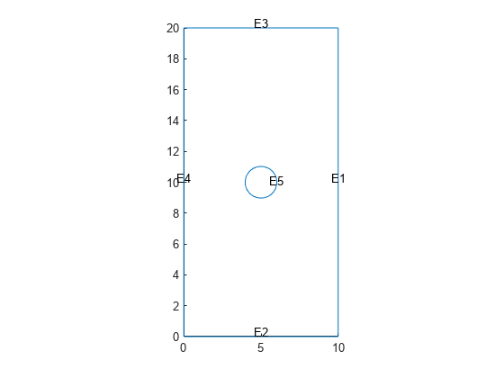
Specify the conductivity of the material.
model.MaterialProperties = ...
    materialProperties(ElectricalConductivity=6e4);
Apply the voltage boundary conditions on the top and bottom edges of the plate.
model.EdgeBC(3) = edgeBC(Voltage=100);
model.EdgeBC(2) = edgeBC(Voltage=200);
Specify the surface current density on the edge representing the hole.
model.EdgeLoad(5) = edgeLoad(SurfaceCurrentDensity=200000);
Generate a mesh.
model = generateMesh(model);
Solve the problem.
R = solve(model);
Plot the electric potential and current density.
figure
pdeplot(R.Mesh,XYData=R.ElectricPotential,ColorMap="jet", ...
               FlowData=[R.CurrentDensity.Jx R.CurrentDensity.Jy])
axis equal

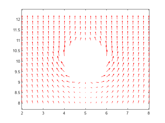
Interpolate the resulting current density to a grid covering the central portion of the geometry.
[X,Y] = meshgrid(2:0.25:8,8:0.25:12);
Jintrp = interpolateCurrentDensity(R,X,Y)
Jintrp =
  FEStruct with properties:

    Jx: [425×1 double]
    Jy: [425×1 double]
Reshape Jintrp.Jx and Jintrp.Jy, and plot the resulting current density.
JintrpX = reshape(Jintrp.Jx,size(X));
JintrpY = reshape(Jintrp.Jy,size(Y));
quiver(X,Y,JintrpX,JintrpY,Color="red")
axis equal
Alternatively, you can specify the grid by using a matrix of query points.
querypoints = [X(:),Y(:)]';
Jintrp = interpolateCurrentDensity(R,querypoints);
Create an femodel object for DC conduction analysis and include a geometry representing a 10-by-10-by-1 solid plate into the model.
model = femodel(AnalysisType="dcConduction", ...
                Geometry="Plate10x10x1.stl");
Plot the geometry.
pdegplot(model.Geometry,FaceLabels="on",FaceAlpha=0.3)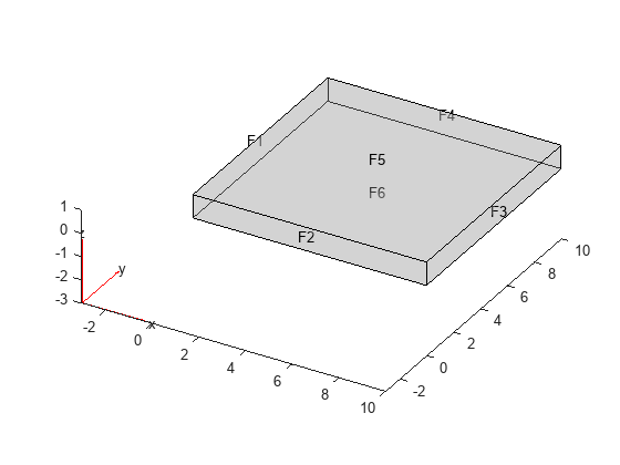
Specify the conductivity of the material.
model.MaterialProperties = ...
    materialProperties(ElectricalConductivity=6e4);
Apply the voltage boundary conditions on the two faces of the plate.
model.FaceBC([1 3]) = faceBC(Voltage=0);
Specify the surface current density on the top of the plate.
model.FaceLoad(5) = faceLoad(SurfaceCurrentDensity=100);
Generate a mesh.
model = generateMesh(model);
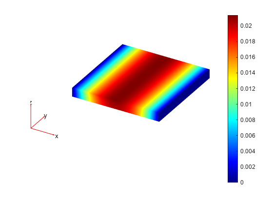
Solve the problem.
R = solve(model);
Plot the electric potential.
figure
pdeplot3D(R.Mesh,ColorMapData=R.ElectricPotential)
Plot the current density.
figure
pdeplot3D(R.Mesh,FlowData=[R.CurrentDensity.Jx, ...
                           R.CurrentDensity.Jy, ...
                           R.CurrentDensity.Jz])
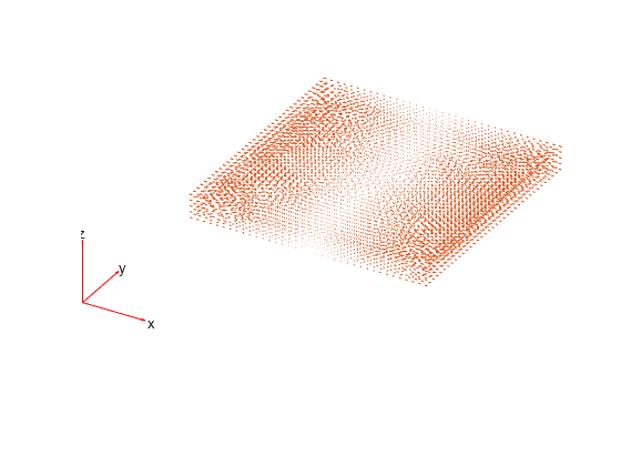
Interpolate the resulting current density to a coarser grid.
[X,Y,Z] = meshgrid(0:10,0:10,0:0.5:1);
Jintrp = interpolateCurrentDensity(R,X,Y,Z)
Jintrp =
  FEStruct with properties:

    Jx: [363×1 double]
    Jy: [363×1 double]
    Jz: [363×1 double]
Reshape Jintrp.Jx, Jintrp.Jy, and Jintrp.Jz.
JintrpX = reshape(Jintrp.Jx,size(X));
JintrpY = reshape(Jintrp.Jy,size(Y));
JintrpZ = reshape(Jintrp.Jz,size(Z));
Plot the resulting current density.
figure
quiver3(X,Y,Z,JintrpX,JintrpY,JintrpZ,Color="red")
Input Arguments
Output Arguments
Version History
Introduced in R2022b