HarmonicResults

For an electromagnetic harmonic analysis problem, find the x- and y-components of the electric field. Solve the problem on a domain consisting of a square with a circular hole.

For the geometry, define a circle in a square, place them in one matrix, and create a set formula that subtracts the circle from the square.

SQ = [3,4,-5,-5,5,5,-5,5,5,-5]';
C = [1,0,0,1]';
C = [C;zeros(length(SQ) - length(C),1)];
gm = [SQ,C];
sf = 'SQ-C';

Create the geometry.

ns = char('SQ','C');
ns = ns';
g = decsg(gm,sf,ns);

Create an femodel object for electromagnetic harmonic analysis with an electric field type. Include the geometry in the model.

model = femodel(AnalysisType="electricHarmonic", ...
                Geometry=g);

Plot the geometry with the edge labels.

pdegplot(model.Geometry,EdgeLabels="on")
xlim([-5.5 5.5])
ylim([-5.5 5.5])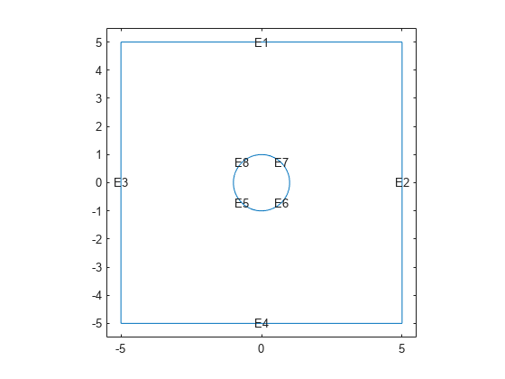

Specify the vacuum permittivity and permeability values as 1.

model.VacuumPermittivity = 1;
model.VacuumPermeability = 1;

Specify the relative permittivity, relative permeability, and conductivity of the material.

model.MaterialProperties = ...
    materialProperties(RelativePermittivity=1, ...
                       RelativePermeability=1, ...
                       ElectricalConductivity=0);

Apply the absorbing boundary condition with a thickness of 2 on the edges of the square. Use the default attenuation rate for the absorbing region.

ffbc = farFieldBC(Thickness=2);
model.EdgeBC(1:4) = edgeBC(FarField=ffbc);

Specify an electric field on the edges of the hole.

E = @(location,state) [1;0]*exp(-1i*2*pi*location.y); 
model.EdgeBC(5:8) = edgeBC(ElectricField=E);

Generate a mesh.

model = generateMesh(model,Hmax=1/2^3);

Solve the model for a frequency of $2\pi$.

result = solve(model,2*pi);

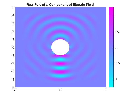
Plot the real part of the x-component of the resulting electric field.

figure
pdeplot(result.Mesh,XYData=real(result.ElectricField.Ex));
title("Real Part of x-Component of Electric Field")

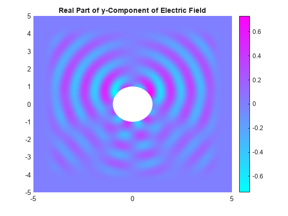
Plot the real part of the y-component of the resulting electric field.

figure
pdeplot(result.Mesh,XYData=real(result.ElectricField.Ey));
title("Real Part of y-Component of Electric Field")