interpolateHarmonicField
Interpolate electric or magnetic field in harmonic result at arbitrary spatial locations
Since R2022a
Syntax
Description
EHintrp = interpolateHarmonicField(harmonicresults,xq,yq)xq and yq.
EHintrp = interpolateHarmonicField(harmonicresults,querypoints)querypoints.
Examples
Solve a simple scattering problem and interpolate the x-component of the resulting electric field. A scattering problem computes the waves reflected by a square object illuminated by incident waves.
Specify the wave number as .
k = 4*pi;
Represent the square surface with a diamond-shaped hole. Define a diamond in a square, place them in one matrix, and create a set formula that subtracts the diamond from the square.
square = [3; 4; -5; -5; 5; 5; -5; 5; 5; -5];
diamond = [2; 4; 2.1; 2.4; 2.7; 2.4; 1.5; 1.8; 1.5; 1.2];
gd = [square,diamond];
ns = char('square','diamond')';
sf = 'square - diamond';
Create the geometry.
g = decsg(gd,sf,ns);
Plot the geometry with the edge labels.
figure;
pdegplot(g,EdgeLabels="on");
xlim([-6,6])
ylim([-6,6])
Create an femodel object for harmonic electromagnetic analysis with the electric field type. Include the geometry into the model.
model = femodel(AnalysisType="electricHarmonic", ...
                Geometry=g);
Specify the vacuum permittivity and permeability values as 1.
model.VacuumPermittivity = 1;
model.VacuumPermeability = 1;
Specify the relative permittivity, relative permeability, and conductivity of the material.
model.MaterialProperties = ...
    materialProperties(RelativePermittivity=1, ...
                       RelativePermeability=1, ...
                       ElectricalConductivity=0);
Apply the absorbing boundary condition on the edges of the square. Specify the thickness and attenuation rate for the absorbing region by using the Thickness, Exponent, and Scaling arguments.
ffbc = farFieldBC(Thickness=2,Exponent=4,Scaling=1);
model.EdgeBC(1:4) = edgeBC(FarField=ffbc);
Apply the boundary condition on the edges of the diamond.
innerBCFunc = @(location,~) [-exp(-1i*k*location.x); ...
                            zeros(1,length(location.x))];
model.EdgeBC(5:8) = edgeBC(ElectricField=innerBCFunc);
Generate a mesh.
model = generateMesh(model,Hmax=0.1);
Solve the harmonic analysis model for the frequency k = .
R = solve(model,k);
Plot the real part of the x-component of the resulting electric field.
u = R.ElectricField;

figure
pdeplot(R.Mesh,XYData=real(u.Ex));
colormap(jet)
axis equal
Interpolate the resulting electric field to a grid covering the portion of the geometry, for x and y from -1 to 4.
v = linspace(-1,4,101);
[X,Y] = meshgrid(v);
Eintrp = interpolateHarmonicField(R,X,Y);
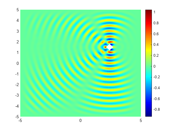
Reshape Eintrp.Ex and plot the x-component of the resulting electric field.
EintrpX = reshape(Eintrp.ElectricField.Ex,size(X));

figure
surf(X,Y,real(EintrpX),LineStyle="none");
view(0,90)
colormap(jet)
axis equal

Interpolate the x-component of the magnetic field in a harmonic analysis of a 3-D model.
Create an femodel object for harmonic electromagnetic analysis with the magnetic field type. Include the geometry representing a plate with a hole into the model.
model = femodel(AnalysisType="magneticHarmonic", ...
                Geometry="PlateHoleSolid.stl");
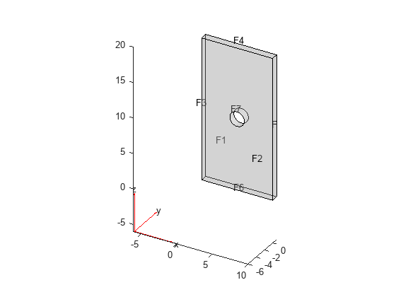
Plot the geometry.
pdegplot(model,FaceLabels="on",FaceAlpha=0.3)
Specify the vacuum permittivity and permeability values in the SI system of units.
model.VacuumPermittivity = 8.8541878128E-12;
model.VacuumPermeability = 1.2566370614E-6;
Specify the relative permittivity, relative permeability, and conductivity of the material.
model.MaterialProperties = ...
    materialProperties(RelativePermittivity=1, ...
                       RelativePermeability=6, ...
                       ElectricalConductivity=60);
Specify the current density for the entire geometry. For harmonic analysis with the magnetic field type, the toolbox uses the curl of the specified current density.
model.CellLoad = cellLoad(CurrentDensity=[1;1;1]);
Apply the absorbing boundary condition with a thickness of 0.1 on the side faces.
ffbc = farFieldBC(Thickness=0.1);
model.FaceBC(3:6) = faceBC(FarField=ffbc);
Specify the magnetic field on the face bordering the round hole in the center of the geometry.
model.FaceBC(7) = faceBC(MagneticField=[1000;0;0]);
Generate a mesh.
model = generateMesh(model);
Solve the model for a frequency of 50.
result = solve(model,50);
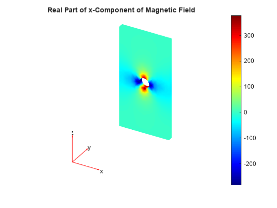
Plot the real part of the x-component of the resulting magnetic field.
u = result.MagneticField;
figure
pdeplot3D(result.Mesh,ColorMapData=real(u.Hx));
colormap jet
title("Real Part of x-Component of Magnetic Field")

Interpolate the resulting magnetic field to a grid covering the central portion of the geometry, for x, y, and z.
x = linspace(3,7,51);
y = linspace(0,1,51);
z = linspace(8,12,51);
[X,Y,Z] = meshgrid(x,y,z);

Hintrp = interpolateHarmonicField(result,X,Y,Z)
Hintrp = struct with fields:
    MagneticField: [1×1 FEStruct]
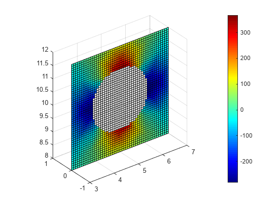
Reshape Hintrp.Hx and plot the x-component of the resulting magnetic field as a slice plot for y = 0.
HintrpX = reshape(Hintrp.MagneticField.Hx,size(X));

figure
slice(X,Y,Z,real(HintrpX),[],0,[],"cubic")
axis equal
colorbar
colormap(jet)

Alternatively, you can specify the grid by using a matrix of query points.
querypoints = [X(:),Y(:),Z(:)]';
Hintrp = interpolateHarmonicField(result,querypoints)
Hintrp = struct with fields:
    MagneticField: [1×1 FEStruct]
Input Arguments
Solution of a harmonic electromagnetic problem, specified as a HarmonicResults
object. Create harmonicresults using the solve function.
x-coordinate query points, specified as a real array.
interpolateHarmonicField evaluates the electric or magnetic field
at the 2-D coordinate points [xq(i) yq(i)] or at the 3-D coordinate
points [xq(i) yq(i) zq(i)] for every index
i.Therefore, xq, yq, and (if
present) zq must have the same number of entries.
interpolateHarmonicField converts the query points to column
vectors xq(:), yq(:), and (if present)
zq(:). It returns electric or magnetic field values as a column
vector of the same size. To ensure that the dimensions of the returned solution are
consistent with the dimensions of the original query points, use
reshape. For example, use EHintrpX =
reshape(EHintrp.Ex,size(xq)).
Example: xq = [0.5 0.5 0.75 0.75]
Data Types: double
y-coordinate query points, specified as a real array.
interpolateHarmonicField evaluates the electric or magnetic field
at the 2-D coordinate points [xq(i) yq(i)] or at the 3-D coordinate
points [xq(i) yq(i) zq(i)] for every index i.
Therefore, xq, yq, and (if present)
zq must have the same number of entries.
interpolateHarmonicField converts the query points to column
vectors xq(:), yq(:), and (if present)
zq(:). It returns electric or magnetic field values as a column
vector of the same size. To ensure that the dimensions of the returned solution are
consistent with the dimensions of the original query points, use
reshape. For example, use EHintrpY =
reshape(EHintrp.Ey,size(yq)).
Example: yq = [1 2 0 0.5]
Data Types: double
z-coordinate query points, specified as a real array.
interpolateHarmonicField evaluates the electric or magnetic field
at the 3-D coordinate points [xq(i) yq(i) zq(i)] for every index
i. Therefore, xq, yq, and
zq must have the same number of entries.
interpolateHarmonicField converts the query points to column
vectors xq(:), yq(:), and
zq(:). It returns electric or magnetic field values as a column
vector of the same size. To ensure that the dimensions of the returned solution are
consistent with the dimensions of the original query points, use
reshape. For example, use EHintrpZ =
reshape(EHintrp.Ez,size(zq)).
Example: zq = [1 1 0 1.5]
Data Types: double
Query points, specified as a real matrix with either two rows for a 2-D geometry or
three rows for a 3-D geometry. interpolateHarmonicField evaluates the
electric or magnetic field at the coordinate points querypoints(:,i)
for every index i, so each column of querypoints
contains exactly one 2-D or 3-D query point.
Example: For a 2-D geometry, querypoints = [0.5 0.5 0.75 0.75; 1 2 0
0.5]
Data Types: double
Output Arguments
Electric or magnetic field at query points, returned as an
FEStruct object with the properties representing the spatial
components of the electric or magnetic field at the query points. For query points that
are outside the geometry, EHintrp.Ex(i),
EHintrp.Ey(i), EHintrp.Ez(i),
EHintrp.Hx(i), EHintrp.Hy(i), and
EHintrp.Hz(i) are NaN. Properties of an
FEStruct object are read-only.
Version History
Introduced in R2022a
MATLAB Command
You clicked a link that corresponds to this MATLAB command:
Run the command by entering it in the MATLAB Command Window. Web browsers do not support MATLAB commands.
选择网站
选择网站以获取翻译的可用内容,以及查看当地活动和优惠。根据您的位置,我们建议您选择:。
您也可以从以下列表中选择网站:
如何获得最佳网站性能
选择中国网站(中文或英文)以获得最佳网站性能。其他 MathWorks 国家/地区网站并未针对您所在位置的访问进行优化。
美洲
- América Latina (Español)
- Canada (English)
- United States (English)
欧洲
- Belgium (English)
- Denmark (English)
- Deutschland (Deutsch)
- España (Español)
- Finland (English)
- France (Français)
- Ireland (English)
- Italia (Italiano)
- Luxembourg (English)
- Netherlands (English)
- Norway (English)
- Österreich (Deutsch)
- Portugal (English)
- Sweden (English)
- Switzerland
- United Kingdom (English)