Set Initial Condition for Model with Fine Mesh Using Solution Obtained with Coarser Mesh

Set initial conditions for a model with a fine mesh by using the coarse-mesh solution from a previous analysis.

Create a PDE model and include the geometry of the built-in function squareg.

model = createpde;
geometryFromEdges(model,@squareg);

Specify the coefficients, apply boundary conditions, and set initial conditions.

specifyCoefficients(model,m=0,d=1,c=5,a=0,f=0.1);
applyBoundaryCondition(model,"dirichlet",Edge=1,u=1);
setInitialConditions(model,10);

Generate a comparatively coarse mesh with the target maximum element edge length of 0.1.

generateMesh(model,Hmax=0.1);

Solve the model for the entire time span of 0 through 0.02 seconds.

tlist = linspace(0,2E-2,20);
Rtotal = solvepde(model,tlist);

Interpolate the solution at the origin for the entire time span.

singleSpanSol = Rtotal.interpolateSolution(0,0,1:numel(tlist)); 

Now solve the model for the first half of the time span. You will use this solution as an initial condition when solving the model with a finer mesh for the second half of the time span.

tlist1 = linspace(0,1E-2,10);
R1 = solvepde(model,tlist1);

Create an interpolant to interpolate the initial condition.

x = model.Mesh.Nodes(1,:)';
y = model.Mesh.Nodes(2,:)';
interpolant = scatteredInterpolant(x,y,R1.NodalSolution(:,end));

Generate a finer mesh by setting the target maximum element edge length to 0.05.

generateMesh(model,Hmax=0.05);

Use the coarse mesh model results as the initial condition for the model with the finer mesh. For the definition of the icFcn function, see Initial Conditions Function.

setInitialConditions(model,@(region) icFcn(region,interpolant));

Solve the model for the second half of the time span.

tlist2 = linspace(1E-2,2E-2,10);
R2 = solvepde(model,tlist2);

Interpolate the solutions at the origin for the first and the second halves of the time span.

multispanSol1 = R1.interpolateSolution(0,0,1:numel(tlist1));
multispanSol2 = R2.interpolateSolution(0,0,1:numel(tlist2));

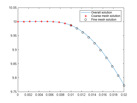
Plot all three solutions at the origin.

figure
plot(tlist,singleSpanSol)
hold on
plot(tlist1, multispanSol1,"r*")
plot(tlist2, multispanSol2,"ko")
legend("Overall solution","Coarse mesh solution", "Fine mesh solution")

function u0 = icFcn(region,interpolant)
u0 = interpolant(region.x',region.y');
end