Thermal and Structural Analysis of Disc Brake
This example shows a quasistatic axisymmetric thermal stress analysis workflow by reproducing the results of the simplified disc brake model discussed in [1]. Disc brakes absorb mechanical energy through friction and transform it into thermal energy, which then dissipates. The example uses a simplified model of a disc brake in a single braking process from a constant initial angular speed to a standstill. The workflow has two steps:
Transient thermal analysis to compute the temperature distribution in the disc using the heat flux from brake pads
Quasistatic structural analysis to compute thermal stresses at several solution times using previously obtained temperature distribution to specify thermal loads
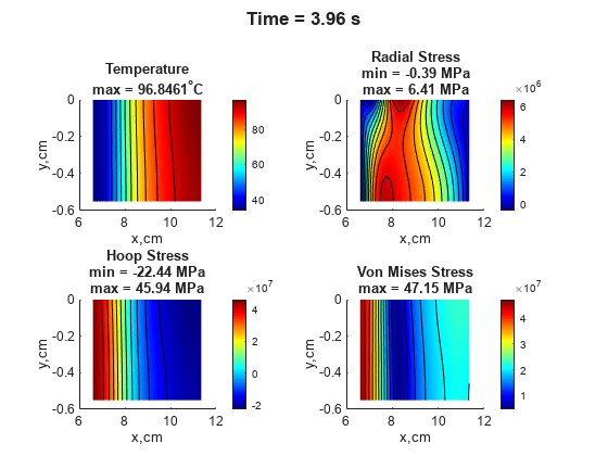
The resulting plots show the temperature distribution, radial stress, hoop stress, and von Mises stress for the corresponding solution times.
Disc Brake Properties and Geometry
Based on the assumptions used in [1], the example reduces the analysis domain to a rectangular region corresponding to the axisymmetric section of the annular disc. Because of the geometric and load symmetry of the disc, the example models only half the thickness of the disc and the effect of one pad. In the following figure, the left edge corresponds to the inner radius of the disc . The right edge corresponds to the outer radius of the disc and also coincides with the outer radius of the pad . The disc experiences pressure from the pad, which generates the heat flux. Instead of modeling the pad explicitly, include its effect in the thermal analysis by specifying this heat flux as a boundary condition from the inner radius of the pad to the outer radius of the pad .

Thermal Analysis: Compute Temperature Distribution
Create a geometry with two adjacent rectangles. The top edge of the longer rectangle (on the right) represents the disc-pad contact region.
R1 = [3,4, [  66,  76.5,  76.5,   66, -5.5, -5.5, 0, 0]/1000]';
R2 = [3,4, [76.5, 113.5, 113.5, 76.5, -5.5, -5.5, 0, 0]/1000]';

gdm = [R1 R2];
ns = char('R1','R2');
g = decsg(gdm,'R1 + R2',ns');
Plot the geometry with the edge and face labels.
figure
pdegplot(g,EdgeLabels="on",FaceLabels="on");

Create a finite element analysis model with the disc brake geometry for transient axisymmetric thermal analysis.
model = femodel(AnalysisType="thermalTransient",Geometry=g);
model.PlanarType = "axisymmetric";
Assign the geometry to the thermal model.
model.Geometry = geometryFromEdges(g);
Generate a mesh. To match the mesh used in [1], use the linear geometric order instead of the default quadratic order.
model = generateMesh(model,Hmax=0.5E-04, ...
                           GeometricOrder="linear");
Specify the thermal material properties of the disc.
alphad = 1.44E-5; % Diffusivity of disc
Kd = 51;
rhod = 7100;
cpd = Kd/rhod/alphad;
model.MaterialProperties = ...
    materialProperties(ThermalConductivity=Kd, ...
                       MassDensity=rhod, ...
                       SpecificHeat=cpd);
Specify the heat flux boundary condition to account for the pad region. For the definition of the qFcn function, see Heat Flux Function.
model.EdgeLoad(6) = edgeLoad(Heat=@qFcn);
Set the initial temperature.
model.FaceIC=faceIC(Temperature=20);
Solve the model for the times used in [1].
tlist = [0 0.1 0.2 1.0 2.0 3.0 3.96];
Rt = solve(model,tlist);
Plot the temperature variation with time at three key radial locations. The resulting plot is comparable to the plot obtained in [1].
iTRd = interpolateTemperature(Rt,[0.1135;0],1:numel(Rt.SolutionTimes));
iTrp = interpolateTemperature(Rt,[0.0765;0],1:numel(Rt.SolutionTimes));
iTrd = interpolateTemperature(Rt,[0.066;0],1:numel(Rt.SolutionTimes));

figure
plot(tlist,iTRd)
hold on
plot(tlist,iTrp)
plot(tlist,iTrd)
title("Temperature Variation with Time at Key Radial Locations")
legend("R_d","r_p","r_d")
xlabel("t, s")
ylabel("T,^{\circ}C")

Structural Analysis: Compute Thermal Stress
Switch the analysis type for the femodel object to static structural.
model.AnalysisType = "structuralStatic";Specify the structural properties of the disc.
model.MaterialProperties = ...
    materialProperties(YoungsModulus=99.97E9, ...
                       PoissonsRatio=0.29, ...
                       CTE=1.08E-5);
Constrain the model to prevent rigid motion.
model.EdgeBC([3,4]) = edgeBC(YDisplacement=0);
Specify the reference temperature that corresponds to the state of zero thermal stress of the model.
model.ReferenceTemperature = 20;
Specify the thermal load by using the transient thermal results Rt. The solution times are the same as in the thermal model analysis. For each solution time, solve the corresponding static structural analysis problem and plot the temperature distribution, radial stress, hoop stress, and von Mises stress. For the definition of the plotResults function, see Plot Results Function. The results are comparable to figure 5 from [1].
for n = 2:numel(Rt.SolutionTimes)
Rt_step = filterByIndex(Rt,n);
model.FaceLoad = faceLoad(Temperature=Rt_step);
R = solve(model);
plotResults(R,Rt,n);
end


Heat Flux Function
This helper function computes the transient value of the heat flux from the pad to the disc. It uses the empirical formula from [1].
function q = qFcn(x,s)
alphad = 1.44E-5; % Diffusivity of disc
Kd = 51; % Conductivity of disc
rhod = 7100; % Density of disc
cpd = Kd/rhod/alphad; % Specific heat capacity of disc

alphap = 1.46E-5; % Diffusivity of pad
Kp = 34.3; % Conductivity of pad
rhop = 4700; % Density of pad
cpp = Kp/rhop/alphap; % Specific heat capacity of pad

f = 0.5; % Coefficient of friction
omega0 = 88.464; % Initial angular velocity
ts = 3.96; % Stopping time
p0 = 1.47E6*(64.5/360); % Pressure only spans 64.5 deg occupied by pad

omegat = omega0*(1 - s.time/ts); % Angular speed over time

eta = sqrt(Kd*rhod*cpd)/(sqrt(Kd*rhod*cpd) + sqrt(Kp*rhop*cpp));
q = (eta)*f*omegat*x.x*p0;
end
Plot Results Function
This helper function plots the temperature distribution, radial stress, hoop stress, and von Mises stress.
function plotResults(R,Rt,tID)
figure
subplot(2,2,1)
pdeplot(Rt.Mesh,XYData=Rt.Temperature(:,tID), ...
               ColorMap="jet",Contour="on")
xt = xticks;
yt = yticks;
xticklabels(100*xt);
yticklabels(100*yt);
xlabel("x,cm")
ylabel("y,cm")
title({'Temperature'; ...
      ['max = ' num2str(max(Rt.Temperature(:,tID))) '^{\circ}C']}, ...
      FontSize=10)

subplot(2,2,2)
pdeplot(R.Mesh,XYData=R.Stress.srr, ...
               ColorMap="jet",Contour="on")
xt = xticks;
yt = yticks;
xticklabels(100*xt);
yticklabels(100*yt);
xlabel("x,cm")
ylabel("y,cm")
title({'Radial Stress'; ...
       ['min = ' num2str(min(R.Stress.srr)/1E6,'%3.2f') ' MPa'];
       ['max = ' num2str(max(R.Stress.srr)/1E6,'%3.2f') ' MPa']}, ...
       FontSize=10)

subplot(2,2,3)
pdeplot(R.Mesh,XYData=R.Stress.sh, ...
               ColorMap="jet",Contour="on")
xt = xticks;
yt = yticks;
xticklabels(100*xt);
yticklabels(100*yt);
xlabel("x,cm")
ylabel("y,cm")
title({'Hoop Stress'; ...
      ['min = ' num2str(min(R.Stress.sh)/1E6,'%3.2f') ' MPa'];
      ['max = ' num2str(max(R.Stress.sh)/1E6,'%3.2f') ' MPa']}, ...
      FontSize=10)

subplot(2,2,4)
pdeplot(R.Mesh,XYData=R.VonMisesStress, ...
               ColorMap="jet",Contour="on")
xt = xticks;
yt = yticks;
xticklabels(100*xt);
yticklabels(100*yt);
xlabel("x,cm")
ylabel("y,cm")
title({'Von Mises Stress'; ...
      ['max = ' num2str(max(R.VonMisesStress)/1E6,'%3.2f') ' MPa']}, ...
      FontSize=10)

sgtitle(['Time = ' num2str(Rt.SolutionTimes(tID)) ' s'],FontWeight="bold")
end
References
[1] Adamowicz, Adam. "Axisymmetric FE Model to Analysis of Thermal Stresses in a Brake Disc." Journal of Theoretical and Applied Mechanics 53, issue 2 (April 2015): 357–370. https://doi.org/10.15632/jtam-pl.53.2.357.