ambgfun

Ambiguity and crossambiguity function

Syntax

afmag = ambgfun(x,Fs,PRF)

[afmag,delay,doppler]
= ambgfun(___)

[afmag,delay,doppler]
= ambgfun(___,Cut="2D")

afmag = ambgfun(x,y,Fs,PRF)

[afmag,delay,doppler]
= ambgfun(___,Cut="2D")

[afmag,delay]
= ambgfun(___,Cut="Doppler")

[afmag,delay]
= ambgfun(___,Cut="Doppler",CutValue=V)

[afmag,doppler]
= ambgfun(___,Cut="Delay")

[afmag,doppler]
= ambgfun(___,Cut="Delay",CutValue=V)

ambgfun(___)

Description

afmag = ambgfun(x,Fs,PRF) returns the magnitude of the normalized ambiguity function for the vector x. Fs is the sampling frequency. PRF is the pulse repetition frequency.

example

[afmag,delay,doppler] = ambgfun(___) or [afmag,delay,doppler] = ambgfun(___,Cut="2D") returns the time delay vector, delay, and the Doppler frequency vector, doppler.

example

afmag = ambgfun(x,y,Fs,PRF) returns the magnitude of the normalized crossambiguity function between pulse x and pulse y. This syntax is equivalent to [afmag,delay,doppler] = ambgfun(___,Cut="2D")

[afmag,delay] = ambgfun(___,Cut="Doppler") returns delays from a zero-Doppler cut through the 2-D normalized ambiguity function magnitude.

example

[afmag,delay] = ambgfun(___,Cut="Doppler",CutValue=V) returns delays from a nonzero Doppler cut through the 2-D normalized ambiguity function magnitude at Doppler values V.

example

[afmag,doppler] = ambgfun(___,Cut="Delay") returns the Doppler values from zero-delay cut through the 2-D normalized ambiguity function magnitude.

[afmag,doppler] = ambgfun(___,Cut="Delay",CutValue=V) returns the Doppler values from a one-dimensional cut through the 2-D normalized ambiguity function magnitude at a delay values V.

ambgfun(___), with no output arguments, plots the ambiguity or crossambiguity function. When is Cut="2D", the function produces a contour plot of the ambiguity function. When Cut="Delay" or Cut="Doppler", the function produces a line plot of the ambiguity function.

example

Examples

collapse all

Plot Ambiguity Function of Rectangular Pulse

Open Live Script

Plot the ambiguity function magnitude of a rectangular pulse.

waveform = phased.RectangularWaveform;
x = waveform();
PRF = waveform.PRF;
[afmag,delay,doppler] = ambgfun(x,waveform.SampleRate,PRF);
contour(delay,doppler,afmag)
xlabel("Delay (seconds)")
ylabel("Doppler Shift (hertz)")

Figure contains an axes object. The axes object with xlabel Delay (seconds), ylabel Doppler Shift (hertz) contains an object of type contour.

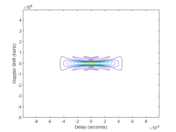
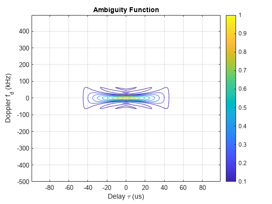
Use the ambgfun function with no output arguments to recreate the plot.

ambgfun(x,waveform.SampleRate,PRF)

Figure contains an axes object. The axes object with title Ambiguity Function, xlabel Delay tau blank (µs), ylabel Doppler f indexOf d baseline blank (kHz) contains an object of type contour.

Plot Autocorrelation Sequences of Rectangular and Linear FM Pulses

Open Live Script

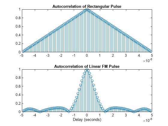
This example shows how to plot zero-Doppler cuts of the autocorrelation sequences of rectangular and linear FM pulses of equal duration. Note the pulse compression exhibited in the autocorrelation sequence of the linear FM pulse.

hrect = phased.RectangularWaveform("PRF",2e4);
hfm = phased.LinearFMWaveform("PRF",2e4);
xrect = hrect();
xfm = hfm();
[ambrect,delayrect] = ambgfun(xrect,hrect.SampleRate,...,
    hrect.PRF,"Cut","Doppler");
[ambfm,delayfm] = ambgfun(xfm,hfm.SampleRate,...,
    hfm.PRF,"Cut","Doppler");

subplot(2,1,1)
stem(delayrect,ambrect)
title("Autocorrelation of Rectangular Pulse")
subplot(2,1,2)
stem(delayfm,ambfm)
xlabel("Delay (seconds)")
title("Autocorrelation of Linear FM Pulse")

Figure contains 2 axes objects. Axes object 1 with title Autocorrelation of Rectangular Pulse contains an object of type stem. Axes object 2 with title Autocorrelation of Linear FM Pulse, xlabel Delay (seconds) contains an object of type stem.

Plot Nonzero-Doppler Cuts of Autocorrelation Sequences

Open Live Script

Plot nonzero-Doppler cuts of the autocorrelation sequences of rectangular and linear FM pulses of equal duration. Both cuts are taken at a 5 kHz Doppler shift. Besides the reduction of the peak value, there is a strong shift in the position of the linear FM peak, evidence of range-doppler coupling.

hrect = phased.RectangularWaveform("PRF",2e4);
hfm = phased.LinearFMWaveform("PRF",2e4);
xrect = hrect();
xfm = hfm();
fd = 5000;
[ambrect,delayrect] = ambgfun(xrect,hrect.SampleRate,...,
    hrect.PRF,"Cut","Doppler","CutValue",fd);
[ambfm,delayfm] = ambgfun(xfm,hfm.SampleRate,...,
    hfm.PRF,"Cut","Doppler","CutValue",fd);

figure
subplot(2,1,1)
stem(delayrect*10^6,ambrect)
title("Autocorrelation of Rectangular Pulse at 5 kHz Doppler Shift")
subplot(2,1,2)
stem(delayfm*10^6,ambfm)
xlabel("Delay (\mu sec)")
title("Autocorrelation of Linear FM Pulse at 5 kHz Doppler Shift")

$Figure contains 2 axes objects. Axes object 1 with title Autocorrelation of Rectangular Pulse at 5 kHz Doppler Shift contains an object of type stem. Axes object 2 with title Autocorrelation of Linear FM Pulse at 5 kHz Doppler Shift, xlabel Delay (\mu sec) contains an object of type stem.$

Plot Crossambiguity Function

Open Live Script

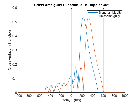
Plot the crossambiguity function between an LFM pulse and a delayed replica. Compare the crossambiguity function with the original ambiguity function. Set the sampling rate to 100 Hz, the pulse width to 0.5 sec, and the pulse repetition frequency to 1 Hz. The delay or lag is 10 samples equal to 100 ms. The bandwidth of the LFM signal is 10 Hz.

fs = 100.0;
bw1 = 10.0;
prf = 1;
nsamp = fs/prf;
pw = 0.5;
nlag = 10;

Create the original waveform and its delayed replica.

waveform1 = phased.LinearFMWaveform("SampleRate",fs,"PulseWidth",1,...
    "SweepBandwidth",bw1,"SweepDirection","Up","PulseWidth",pw,"PRF",prf);
wav1 = waveform1();
wav2 = [zeros(nlag,1);wav1(1:(end-nlag))];

Plot the ambiguity and crossambiguity functions.

ambgfun(wav1,fs,prf,"Cut","Doppler","CutValue",5)
hold on
ambgfun(wav1,wav2,fs,[prf,prf],"Cut","Doppler","CutValue",5)
hold off
legend("Signal ambiguity","Crossambiguity")

Figure contains an axes object. The axes object with title Crossambiguity Function, 5 Hz Doppler Cut, xlabel Delay tau blank (ms), ylabel Crossambiguity Function contains 2 objects of type line. These objects represent Signal ambiguity, Crossambiguity.

Input Arguments

collapse all

`x` — Input pulse waveform
complex-valued row or column vector

Input pulse waveform, specified as a complex-valued row or column vector.

Example: wf = phased.LinearFMWaveform; wf()

Data Types: dounle | single

`y` — Second input pulse waveform
complex-valued row or column vector

Second input pulse waveform, specified as a complex-valued row or column vector.

Example: wf = phased.RectangularWaveform; wf()

Data Types: dounle | single

`Fs` — Sample frequency (Hz)
positive scalar

Sample frequency, specified as a positive scalar. Units are in Hz.

Example: wf = phased.LinearFMWaveform; wf.SampleRate

Data Types: dounle | single

`PRF` — Pulse repetition frequency (Hz)
positive scalar

Pulse repetition frequency, specified as a positive scalar. Units are in Hz.

Example: wf = phased.LinearFMWaveform; wf.PRF

Data Types: dounle | single

Name-Value Arguments

collapse all

Specify optional pairs of arguments as Name1=Value1,...,NameN=ValueN, where Name is the argument name and Value is the corresponding value. Name-value arguments must appear after other arguments, but the order of the pairs does not matter.

Before R2021a, use commas to separate each name and value, and enclose Name in quotes.

Example: Cut="Doppler",CutValue=10 specifies that a vector of ambiguity function values be produced at a Doppler shift of 10 Hz.

`Cut` — Direction of one-dimensional cut through ambiguity function
`"2D"` (default) | `"Delay"` | `"Doppler"`

Used to generate an ambiguity surface or one-dimensional cut through the ambiguity diagram. The value "2D" generates a surface plot of the two-dimensional ambiguity function. The direction of the one-dimensional cut is determined by setting the value of "Cut" to "Delay" or "Doppler".

The choice of "Delay" generates a cut at zero time delay. In this case, the second output argument of ambgfun contains the ambiguity function values at Doppler-shifted values. You can create a cut at nonzero time delay using the name-value pair "CutValue".

The choice of "Doppler" generates a cut at zero Doppler shift. In this case, the second output argument of ambgfun contains the ambiguity function values at time-delayed values. You can create cut at nonzero Doppler using the name-value pair "CutValue".

Data Types: char | string

`CutValue` — Optional time delays or Doppler-shifts at which ambiguity function cuts is taken
0 (default) | real-valued scalar | length-K real-valued vector

Cut values, specified as a real-valued scalar or length-K real-valued vector. When setting the name-value pair "Cut" to "Delay" or "Doppler", you can set "CutValue" to specify cross-sections that may not coincide with either zero time delay or zero Doppler shift. However, "CutValue" cannot be used when "Cut" is set to "2D".

When "Cut" is set to "Delay", "CutValue" is the time delay at which the cut is taken. If '"Cut" is "Delay", the entries in V should be between -T and T where T is the duration of the waveform X in seconds. In this case the output afmag is an M-by-K matrix, where M is the number of Doppler shifts. Time delay units are in seconds.
When "Cut" is set to "Doppler", "CutValue" is the Doppler shift at which the cut is taken. If "Cut" is '"Doppler'", the entries in V should be between -Fs/2 and Fs/2, where Fs is the sampling frequency in Hz. In this case the output afmag is a K-by-N matrix, where N is the number of time delays. Doppler units are in Hz.

Example: CutValue=10.0

Dependencies

To enable this Name-Value argument, set the value of the Name-Value argument Vto "Delay" or "Doppler".

Data Types: double

Output Arguments

collapse all

`afmag` — Normalized ambiguity or crossambiguity function magnitudes
matrix

Normalized ambiguity or crossambiguity function magnitudes, returned as a matrix. afmag is an M-by-N matrix where M is the number of Doppler frequencies and N is the number of time delays.

`delay` — Time delays
vector

Time delays, returned as a vector. delay is an N-by-1 vector of time delays.

For the ambiguity function, if N_x is the length of signal x, then the delay vector consist of N = 2N_x – 1 samples in the range, –(N_x/2) – 1,...,(N_x/2) – 1).

For the crossambiguity function, let N_y be the length of the second signal. The time delay vector consists of N = N_x+ N_y– 1 equally spaced samples. For an even number of delays, the delay sample times are –(N/2 – 1)/Fs,...,(N/2 – 1))/Fs. For an odd number of delays, if N_f= floor(N/2), the delay sample times are –N_f/Fs,...,(N_f – 1)/Fs.

`doppler` — Doppler frequencies
vector

Doppler frequencies, returned as a vector. doppler is an M-by-1 vector of Doppler frequencies. The Doppler frequency vector consists of M = 2^{ceil(log2
N)} equally-spaced samples. Frequencies are –F_s/2,...,F_s/2-F_s/M.

More About

collapse all

Normalized Ambiguity Function

The normalized ambiguity function is

$\begin{array}{l} A (t, f_{d}) = \frac{1}{E_{x}} | \int_{- \infty}^{\infty} x (u) e^{j 2 π f_{d} u} x^{*} (u - t) d u | \\ E_{x} = \int_{- \infty}^{\infty} x (u) x^{*} (u) d u \end{array}$

where E_x is the squared norm of the signal, x(t), t is the time delay, and f_d is the Doppler shift. The asterisk (*) denotes the complex conjugate. The ambiguity function describes the effects of time delays and Doppler shifts on the output of a matched filter.

The magnitude of the ambiguity function achieves maximum value at (0,0). At this point, there is perfect correspondence between the received waveform and the matched filter. The maximum value of the normalized ambiguity function is one.

The magnitude of the ambiguity function at zero time delay and Doppler shift, $| A (0, 0) |,$ is the matched filter output when the received waveform exhibits the time delay and Doppler shift for which the matched filter is designed. Nonzero values of the time delay and Doppler shift variables indicate that the received waveform exhibits mismatches in time delay and Doppler shift from the matched filter.

The function

$\begin{array}{l} A (t, f_{d}) = \frac{1}{\sqrt{E_{x} E_{y}}} | \int_{- \infty}^{\infty} x (u) e^{j 2 π f_{d} u} y^{*} (u - t) d u | \\ E_{x} = \int_{- \infty}^{\infty} x (u) x^{*} (u) d u \\ E_{y} = \int_{- \infty}^{\infty} y (u) y^{*} (u) d u \end{array}$

represents the crossambiguity between two different signals. Note that the peak of the crossambiguity function is not necessarily unity.

Extended Capabilities

expand all

C/C++ Code Generation
Generate C and C++ code using MATLAB® Coder™.

Usage notes and limitations:

Does not support variable-size inputs.
Supported only when output arguments are specified.

References

[1] Levanon, N. and E. Mozeson. Radar Signals. Hoboken, NJ: John Wiley & Sons, 2004.

[2] Mahafza, B. R., and A. Z. Elsherbeni. MATLAB^® Simulations for Radar Systems Design. Boca Raton, FL: CRC Press, 2004.

[3] Richards, M. A. Fundamentals of Radar Signal Processing. New York: McGraw-Hill, 2005.

GPU Arrays
Accelerate code by running on a graphics processing unit (GPU) using Parallel Computing Toolbox™.

Version History

Introduced in R2011a

ambgfun

Syntax

Description

Examples

Plot Ambiguity Function of Rectangular Pulse

Plot Autocorrelation Sequences of Rectangular and Linear FM Pulses

Plot Nonzero-Doppler Cuts of Autocorrelation Sequences

Plot Crossambiguity Function

Input Arguments

`x` — Input pulse waveform
complex-valued row or column vector

`y` — Second input pulse waveform
complex-valued row or column vector

`Fs` — Sample frequency (Hz)
positive scalar

`PRF` — Pulse repetition frequency (Hz)
positive scalar

Name-Value Arguments

`Cut` — Direction of one-dimensional cut through ambiguity function
`"2D"` (default) | `"Delay"` | `"Doppler"`

`CutValue` — Optional time delays or Doppler-shifts at which ambiguity function cuts is taken
0 (default) | real-valued scalar | length-K real-valued vector

Dependencies

Output Arguments

`afmag` — Normalized ambiguity or crossambiguity function magnitudes
matrix

`delay` — Time delays
vector

`doppler` — Doppler frequencies
vector

More About

Normalized Ambiguity Function

Extended Capabilities

C/C++ Code Generation
Generate C and C++ code using MATLAB® Coder™.

References

GPU Arrays
Accelerate code by running on a graphics processing unit (GPU) using Parallel Computing Toolbox™.

Version History

See Also

Functions

Objects

ambgfun

Syntax

Description

Examples

Plot Ambiguity Function of Rectangular Pulse

Plot Autocorrelation Sequences of Rectangular and Linear FM Pulses

Plot Nonzero-Doppler Cuts of Autocorrelation Sequences

Plot Crossambiguity Function

Input Arguments

x — Input pulse waveform complex-valued row or column vector

y — Second input pulse waveform complex-valued row or column vector

Fs — Sample frequency (Hz) positive scalar

PRF — Pulse repetition frequency (Hz) positive scalar

Name-Value Arguments

Cut — Direction of one-dimensional cut through ambiguity function "2D" (default) | "Delay" | "Doppler"

CutValue — Optional time delays or Doppler-shifts at which ambiguity function cuts is taken 0 (default) | real-valued scalar | length-K real-valued vector

Dependencies

Output Arguments

afmag — Normalized ambiguity or crossambiguity function magnitudes matrix

delay — Time delays vector

doppler — Doppler frequencies vector

More About

Normalized Ambiguity Function

Extended Capabilities

C/C++ Code Generation Generate C and C++ code using MATLAB® Coder™.

References

GPU Arrays Accelerate code by running on a graphics processing unit (GPU) using Parallel Computing Toolbox™.

Version History

See Also

Functions

Objects

`x` — Input pulse waveform
complex-valued row or column vector

`y` — Second input pulse waveform
complex-valued row or column vector

`Fs` — Sample frequency (Hz)
positive scalar

`PRF` — Pulse repetition frequency (Hz)
positive scalar

`Cut` — Direction of one-dimensional cut through ambiguity function
`"2D"` (default) | `"Delay"` | `"Doppler"`

`CutValue` — Optional time delays or Doppler-shifts at which ambiguity function cuts is taken
0 (default) | real-valued scalar | length-K real-valued vector

`afmag` — Normalized ambiguity or crossambiguity function magnitudes
matrix

`delay` — Time delays
vector

`doppler` — Doppler frequencies
vector

C/C++ Code Generation
Generate C and C++ code using MATLAB® Coder™.

GPU Arrays
Accelerate code by running on a graphics processing unit (GPU) using Parallel Computing Toolbox™.