lcmvweights
Narrowband linearly constrained minimum variance (LCMV) beamformer weights
Description
wt = lcmvweights(constr,resp,cov)wt, for a phased array. When applied
to the elements of the array, these weights steer the response of
the array toward a specific arrival direction or set of directions.
LCMV beamforming requires that the beamformer response to signals
from a direction of interest are passed with specified gain and phase
delay. However, power from interfering signals and noise from all
other directions is minimized. Additional constraints may be imposed
to specifically nullify output power coming from known directions.
The constraints are contained in the matrix, constr.
Each column of constr represents a separate constraint
vector. The desired response to each constraint is contained in the
response vector, resp. The argument cov is
the sensor spatial covariance matrix. All elements in the sensor array
are assumed to be isotropic.
Examples
Construct a 10-element half-wavelength-spaced line array. Then, compute the LCMV weights for a desired arrival direction of 0 degrees azimuth. Impose three direction constraints: a null at -40 degrees, a unit desired response in the arrival direction 0 degrees, and another null at 20 degrees. The sensor spatial covariance matrix includes two signals arriving from -60 and 60 degrees and -10 dB isotropic white noise.
N = 10;
d = 0.5;
elementPos = (0:N-1)*d;
sv = steervec(elementPos,[-40 0 20]);
resp = [0 1 0]';
Sn  = sensorcov(elementPos,[-60 60],db2pow(-10));
Compute the beamformer weights.
w = lcmvweights(sv,resp,Sn);
Plot the array pattern for the computed weights.
vv = steervec(elementPos,[-90:90]);
plot([-90:90],mag2db(abs(w'*vv)))
grid on
axis([-90,90,-50,10]);
xlabel('Azimuth Angle (degrees)');
ylabel('Normalized Power (dB)');
title('LCMV Array Pattern');
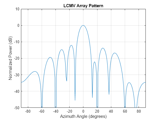
The above figure shows that maximum gain is attained at 0 degrees as expected. In addition, the constraints impose nulls at -40 and 20 degrees and these can be seen in the plot. The nulls at -60 and 60 degrees arise from the fundamental property of the LCMV beamformer of suppressing the power contained in the two plane waves that contributed to the sensor spatial covariance matrix.
Input Arguments
Output Arguments
More About
References
[1] Van Trees, H.L. Optimum Array Processing. New York, NY: Wiley-Interscience, 2002.
[2] Johnson, Don H. and D. Dudgeon. Array Signal Processing. Englewood Cliffs, NJ: Prentice Hall, 1993.
[3] Van Veen, B.D. and K. M. Buckley. “Beamforming: A versatile approach to spatial filtering”. IEEE ASSP Magazine, Vol. 5 No. 2 pp. 4–24.
Extended Capabilities
Version History
Introduced in R2013a
See Also
cbfweights | mvdrweights | sensorcov | steervec | phased.LCMVBeamformer