Main Content

phased.AlphaBetaFilter

Alpha-beta filter for object tracking

Description

The phased.AlphaBetaFilter object creates an alpha-beta filter designed for object tracking. Use this tracker for platforms that follow a linear motion model and have a linear measurement model. Linear motion is defined by constant velocity or constant acceleration. Use the filter to predict the future location of an object, to reduce noise for a detected location, or to help associate multiple objects with their tracks.

Creation

Description

abf = phased.AlphaBetaFilter creates an alpha-beta filter for a discrete time, 2-D constant velocity system. The motion model of the filter corresponds to setting the MotionModel property to '2D Constant Velocity'. In this case, the filter state takes the form [x; vx; y; vy].

abf = phased.AlphaBetaFilter(Name=Value) specifies the properties of the filter using one or more Name=Value pair arguments. Any unspecified properties take default values.

example

Properties

expand all

Model of target motion, specified as a character vector or string. Specifying 1D, 2D or 3D sets the dimensions of the targets motion. Specifying Constant Velocity assumes that the target motion has constant velocity at each simulation step. Specifying Constant Acceleration assumes that the target motion has constant acceleration at each simulation step.

Data Types: char | string

Filter state, specified as a scalar or a real-valued M-element vector. A scalar input is extended to an M-element vector. The state vector is the concatenated states from each dimension.

The state vectors for each motion model are column vectors:

MotionModel PropertyState Vector
'1D Constant Velocity'[x; vx]
'2D Constant Velocity'[x; vx; y; vy]
'3D Constant Velocity'[x; vx; y; vy; z; vz]
'1D Constant Acceleration'[x; vx; ax]
'2D Constant Acceleration'[x; vx; ax; y; vy; ay]
'3D Constant Acceleration'[x; vx; ax; y; vy; ay; z; vz; az]

where, for example, vx denotes velocity in the x-direction and ax denotes acceleration in the x-direction.

Example: [200;0.2;150;0.1;0;0.25]

Data Types: double

State error covariance, specified as an M-by-M matrix where M is the size of the filter state. A scalar input is extended to an M-by-M matrix. The covariance matrix represents the uncertainty in the filter state.

Example: eye(6)

Process noise covariance, specified as a scalar or an D-by-D matrix where D is the dimensionality of motion. For example, if MotionModel is '2D Constant Velocity, then D = 2. A scalar input is extended to an D-by-D matrix.

Example: [20 0.1; 0.1 1]

Measurement noise covariance, specified as a scalar or an D-by-D matrix where D is the dimensionality of motion. For example, if MotionModel is '2D Constant Velocity, then D = 2. A scalar input is extended to an M-by-M matrix.

Example: [20 0.1; 0.1 1]

Alpha-beta filter coefficients, specified as a scalar or row vector of real values. Any scalar input is extended to a row vector. If you specify constant velocity in the MotionModel property, the coefficients are [alpha beta]. If you specify constant acceleration in the MotionModel property, the coefficients are [alpha beta gamma].

Example: [20 0.1]

Object Functions

predictPredict the state and state estimation error covariance
correctCorrect the state and state estimation error covariance
distanceDistances between measurements and predicted measurements
likelihoodLikelihood of measurement
cloneCreate identical object

Examples

collapse all

Apply the alpha-beta filter to track a target moving at constant velocity along the x-axis.

T = 0.1;
V0 = 100;
N = 100;
plat = phased.Platform('MotionModel','Velocity', ...
    'VelocitySource','Input port','InitialPosition',[100;0;0]);
abfilt = phased.AlphaBetaFilter('MotionModel','1D Constant Velocity');
Z = zeros(1,N);
Zp = zeros(1,N);
Zc = zeros(1,N);
for m = 1:N
    pos = plat(T,[100+20*randn;0;0]);
    Z(m) = pos(1);
    [~,~,Zp(m)] = predict(abfilt,T);
    [~,~,Zc(m)] = correct(abfilt,Z(m));
end
t = (0:N-1)*T;
plot(t,Z,t,Zp,t,Zc)
xlabel('Time (s)')
ylabel('Position (m)')
legend('True Track','Predicted Track','Corrected Track', ...
    'Location','Best')

Figure contains an axes object. The axes object with xlabel Time (s), ylabel Position (m) contains 3 objects of type line. These objects represent True Track, Predicted Track, Corrected Track.

Apply the alpha-beta filter to track a target moving at constant acceleration along the x-axis.

T = 0.1;
a0 = 100;
N = 100;
plat = phased.Platform('MotionModel','Acceleration', ...
    'AccelerationSource','Input port','InitialPosition',[100;0;0]);
abfilt = phased.AlphaBetaFilter( ...
    'MotionModel','1D Constant Acceleration', ...
    'Coefficients',[0.5 0.5 0.1]);
Z = zeros(1,N);  
Zp = zeros(1,N);
Zc = zeros(1,N);
for m = 1:N
    pos = plat(T,[100+20*randn;0;0]);
    Z(m) = pos(1);
    [~,~,Zp(m)] = predict(abfilt,T);
    [~,~,Zc(m)] = correct(abfilt,Z(m));
end
t = (0:N-1)*T;
plot(t,Z,t,Zp,t,Zc)
xlabel('Time (s)')
ylabel('Position (m)');
legend('True Track','Predicted Track','Corrected Track', ...
    'Location','Best');

Figure contains an axes object. The axes object with xlabel Time (s), ylabel Position (m) contains 3 objects of type line. These objects represent True Track, Predicted Track, Corrected Track.

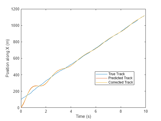
Apply the alpha-beta filter to track a target moving at constant velocity in three dimensions.

T = 0.1;
V0 = 100;
N = 100;
plat = phased.Platform('MotionModel','Velocity', ...
    'VelocitySource','Input port','InitialPosition',[100;0;0]);
abfilt = phased.AlphaBetaFilter('MotionModel', ...
    '3D Constant Velocity','State',zeros(6,1));
Z = zeros(3,N);
Zp = zeros(3,N);
Zc = zeros(3,N);
for m = 1:N
    Z(:,m) = plat(T,[V0+20*randn;0;0]);
    [~,~,Zp(:,m)] = predict(abfilt,T);
    [~,~,Zc(:,m)] = correct(abfilt,Z(:,m));
end
t = (0:N-1)*T;
plot(t,Z(1,:),t,Zp(1,:),t,Zc(1,:))
xlabel('Time (s)')
ylabel('Position along X (m)')
legend('True Track','Predicted Track','Corrected Track', ...
    'Location','Best')

Figure contains an axes object. The axes object with xlabel Time (s), ylabel Position along X (m) contains 3 objects of type line. These objects represent True Track, Predicted Track, Corrected Track.

References

[1] Blackman, Multiple-Target Tracking with Radar Applications, Artech House, 1986.

[2] Bar-Shalom et al., Estimation with Applications to Tracking and Navigation, Theory, Algorithms, and Software. John Wiley & Sons, 2001.

Extended Capabilities

C/C++ Code Generation
Generate C and C++ code using MATLAB® Coder™.

Version History

Introduced in R2018b