plotResponse
System object: phased.HeterogeneousConformalArray
Namespace: phased
Plot response pattern of array
Syntax
plotResponse(H,FREQ,V)

plotResponse(H,FREQ,V,Name,Value)

hPlot = plotResponse(___)
Description
plotResponse( plots
the array response pattern along the azimuth cut, where the elevation
angle is 0. The operating frequency is specified in H,FREQ,V)FREQ.
The propagation speed is specified in V.
plotResponse(
plots the array response with additional options specified by one
or more H,FREQ,V,Name,Value)Name,Value pair arguments.
hPlot = plotResponse(___)
Input Arguments
| |
| |
|
Name-Value Arguments
Examples
This example shows how to construct an 8-element uniform circular array (UCA) with two different antenna patterns.
element1 = phased.CosineAntennaElement('CosinePower',1.5);
element2 = phased.CosineAntennaElement('CosinePower',1.8);
N = 8;
azang = (0:N-1)*360/N-180;
array = phased.HeterogeneousConformalArray( ...
    'ElementPosition',0.4*[zeros(1,N); cosd(azang); sind(azang)], ...
    'ElementNormal',zeros(2,N),'ElementSet',{element1,element2}, ...
    'ElementIndices',[1 1 1 1 2 2 2 2]);
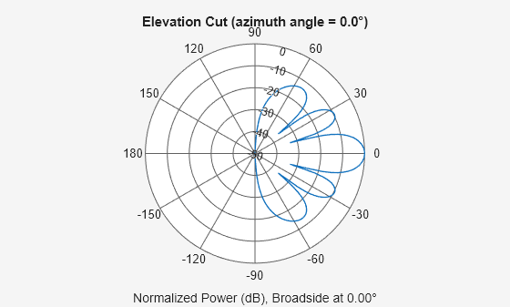
Plot the array elevation response when the operating frequency is 1 GHz and the wave propagation speed is the speed of light.
c = physconst('LightSpeed');
fc = 1e9;
pattern(array,fc,0.0,-90:90,'PropagationSpeed',c,'CoordinateSystem','polar', ...
    'Type','powerdb')
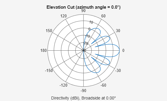
Plot the directivity.
pattern(array,fc,0.0,-90:90,'PropagationSpeed',c,'CoordinateSystem','polar', ...
    'Type','directivity')
This example shows how to construct a 24-element disk array using elements with two different antenna patterns and plot its response.
sElement1 = phased.CosineAntennaElement('CosinePower',1.5);
sElement2 = phased.CosineAntennaElement('CosinePower',1.8);
N = 8; azang = (0:N-1)*360/N-180;
p0 = [zeros(1,N);cosd(azang);sind(azang)];
posn = [0.6*p0, 0.4*p0, 0.2*p0];
sArray1 = phased.HeterogeneousConformalArray(...
    'ElementPosition',posn,...
    'ElementNormal', zeros(2,3*N),...
    'ElementSet',{sElement1,sElement2},...
    'ElementIndices',[1 1 1 1 1 1 1 1,...
    1 1 1 1 1 1 1 1,...
    2 2 2 2 2 2 2 2]);
Show the array.
viewArray(sArray1);

Plot the elevation response of this array using uniform weights on the elements and also a tapered set of weights set by the Weights parameter. Using the ElevationAngles parameter, restrict the plot of the response from -60 to 60 degrees in 0.1 degree increments. Assume the operating frequency is 1 GHz and the wave propagation speed is the speed of light.
c = physconst('LightSpeed');
fc = 1e9;
wts1 = ones(3*N,1);
wts1 = wts1/sum(abs(wts1));
wts2 = [0.5*ones(N,1); 0.7*ones(N,1); 1*ones(N,1)];
wts2 = wts2/sum(abs(wts2));
plotResponse(sArray1,fc,c,'RespCut','El',...
    'Format','Polar',...
    'ElevationAngles',[-60:0.1:60],...
    'Weights',...
    [wts1,wts2],...
    'Unit','db');
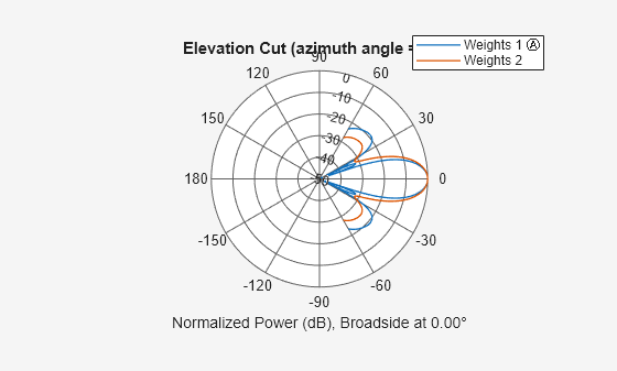
As expected, the tapered weights broaden the mainlobe and reduce the sidelobes.