Main Content

sidelobelevel

Peak and integrated side-lobe levels

Since R2024b

    Description

    sidelobelevel returns the peak sidelobe level of a set of vector data that can represent, for example, autocorrelation functions, array beam patterns, or matched filter output, or any data that can have a peak-and-lobe shape. The data must be dB-scaled data. The function can optionally return integrated sidelobe levels.

    psl = sidelobelevel(Y) calculates the peak sidelobe level (PSL), psl, from an N-element vector Y containing dB values. The input Y may represent data from an autocorrelation function, array beam pattern, matched filter output, or other dB-scaled data.

    example

    psl = sidelobelevel(Y,SmoothingFactor=sf) applies a smoothing window to the data with size factor sf. The smoothing window size factor can range from 0 to 1. Smaller values result in less smoothing, while values closer to 1 result in more smoothing. The default is 0 (no smoothing). Smoothing utilizes a moving Gaussian-weighted window to reduce local variations in Y improving accurate identification of the mainlobe and sidelobes in the presence of noise and distortion.

    psl = sidelobelevel(Y,MaxRipple=mr) specifies the maximum ripple height mr, as a non-negative scalar. Ripples smaller than mr dB are disregarded in mainlobe and sidelobe detection. The default mr value is 0 dB.

    [isl,isl] = sidelobelevel(Y,___) also returns the integrated sidelobe level isl (ISL).

    sidelobelevel(Y,___) produces a plot of the input data, Y, highlighting the estimated mainlobe and sidelobe regions.

    Examples

    collapse all

    Compute the peak and integrated sidelobe levels of the array pattern of a 32-element uniform linear array (ULA) of cosine antenna elements. The array operating frequency is 300 HMz. Apply a Hamming taper to the array.

    N = 32;
    fc = 300e6;

    Compute the operating wavelength.

    lambda = freq2wavelen(fc);

    Construct the ULA using cosine antenna elements.

    element = phased.CosineAntennaElement(CosinePower=[8,8]);
    ula = phased.ULA(N,lambda/2,'Element',element,'Taper',hamming(N));

    Compute the array pattern.

    az = -90:0.1:90;
    pat = pattern(ula,fc,az,0,'Type','powerdb', ...
         'CoordinateSystem','rectangular','Normalize',true);

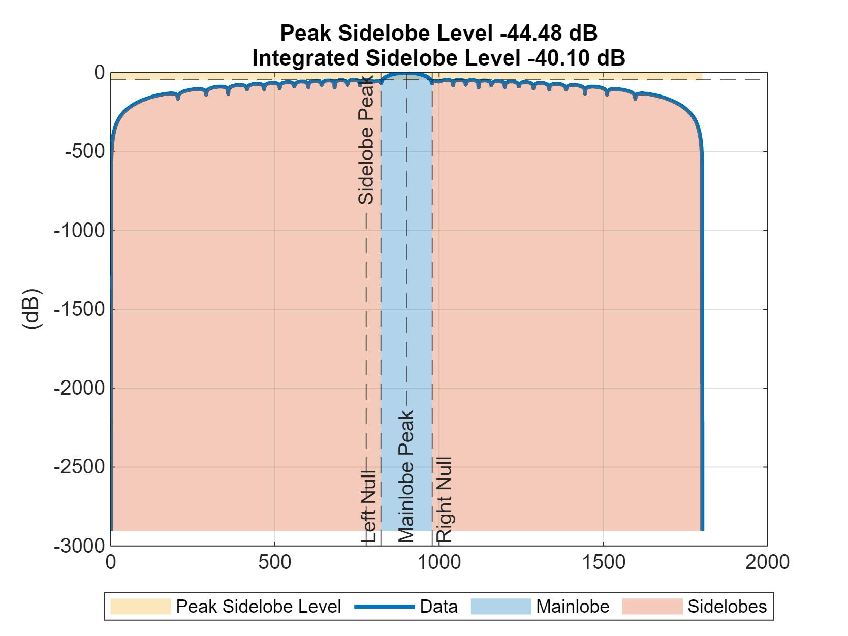
    Compute and display the array sidelobe levels.

    [psl,isl]=sidelobelevel(pat)
    psl = 
    -44.4832
    
    isl = 
    -40.1004
    
    sidelobelevel(pat)

    Figure contains an object of type phased.internal.sidelobelevelchart.

    Input Arguments

    collapse all

    Vector data, specified as an N-element real-valued vector. The Y vector can represent various sources of data such as autocorrelation functions, array beam patterns, matched filter outputs, or other dB-scaled characteristic. Units are in dB.

    Data Types: single | double

    Smoothing factor, specified as a nonnegative scalar between 0 and 1. Use this argument with the SmoothingFactor Name-Value pair. Units are dimensionless.

    Example: SmoothingFactor=0.5

    Data Types: single | double

    Maximum ripple, specified as nonnegative scalar. Use this argument with the MaxRipple Name-Value pair. Units are in dB.

    Example: MaxRipple = 10

    Data Types: single | double

    Output Arguments

    collapse all

    Peak sidelobe level, returned as a scalar. Units are in dB.

    Integrated sidelobe level, returned as a scalar. Units are in dB.

    More About

    collapse all

    Version History

    Introduced in R2024b