whiteningmat

Whitening transformation of covariance matrix

Since R2026a

Syntax

W = whiteningmat(Ncov)

w = whiteningmat(Ncov,OutputNoisePower=pow)

Description

W = whiteningmat(Ncov) returns the transformation matrix W that whitens the noise covariance matrix Ncov of a signal. A whitening transformation converts the data covariance matrix into a scaled identity matrix, effectively whitening the data.

example

w = whiteningmat(Ncov,OutputNoisePower=pow) also specifies the whitened output noise power pow using the OutputNoisePower Name-value argument.

example

Examples

collapse all

Plot Whitened Covariance Matrix

Open Live Script

Apply the whiteningmat function to a 10-by-10 stationary colored noise covariance matrix. Plot the covariance matrix magnitude before and after whitening.

rng default

Specify the covariance matrix dimension N=10 and the number of independent noise samples M=1000.

N = 10;
M = 1000;

Generate a Toeplitz matrix representing the covariance of stationary noise with a constant correlation structure.

corr_coeff = 0.6;
alpha = 5;
indices = 0:N-1;
R = alpha*corr_coeff.^ abs(indices - indices');

Generate colored noise samples and the estimated original covariance matrix using Cholesky factorization.

L = chol(R,'lower');
x = L*randn(N,M);
R_est = cov(x');

Plot estimated original covariance matrix.

figure
imagesc(R_est)
colorbar
title('Estimated Original Covariance Matrix Magnitude')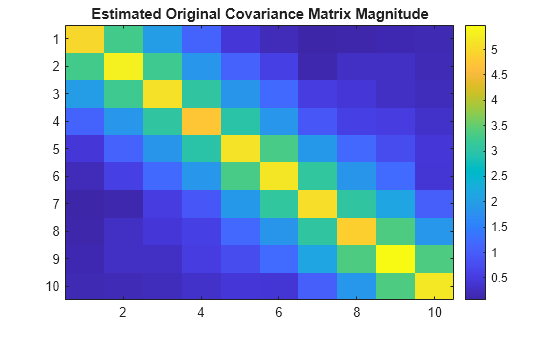

Figure contains an axes object. The axes object with title Estimated Original Covariance Matrix Magnitude contains an object of type image.

Apply the whitening transformation.

outnoisevar = 1;
w = whiteningmat(R_est,OutputNoisePower=outnoisevar);
x_whiten = w*x;
R_whiten_est = cov(x_whiten.');

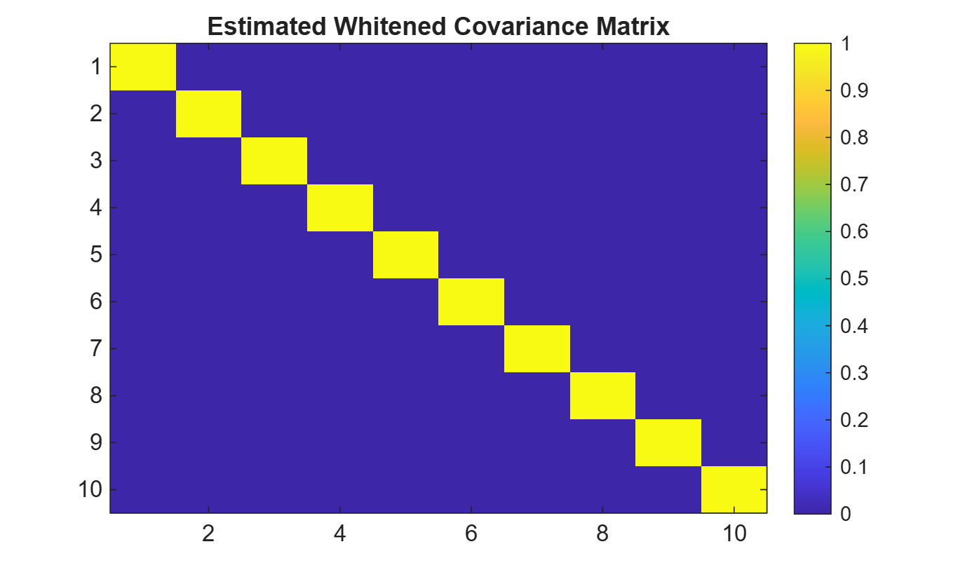
Plot the estimated whitened covariance matrix.

figure
imagesc(R_whiten_est)
colorbar
title('Estimated Whitened Covariance Matrix')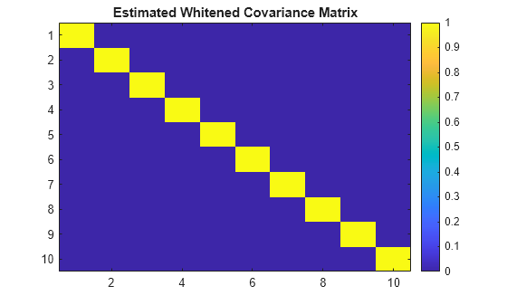

Figure contains an axes object. The axes object with title Estimated Whitened Covariance Matrix contains an object of type image.

Plot Whitened Complex Covariance Matrix

Open Live Script

Apply the whiteningmat function to a 500-by-500 pink noise covariance matrix. Plot the covariance matrix magnitude before and after whitening.

rng default

Specify the covariance matrix dimension N = 500 and the number of independent channels M = 10000.

N = 500;
M = 1e4;
color = "pink";

Configure a colored noise generator and then generate the noise.

pinkNoiseGen = dsp.ColoredNoise(Color=color, ...
    SamplesPerFrame=N,NumChannels=M);
sig = pinkNoiseGen() + 1i*pinkNoiseGen();

Plot estimated original covariance matrix.

covMatrix = cov(sig');
figure
imagesc(abs(covMatrix))
colorbar
title("Estimated Original Covariance Matrix Magnitude")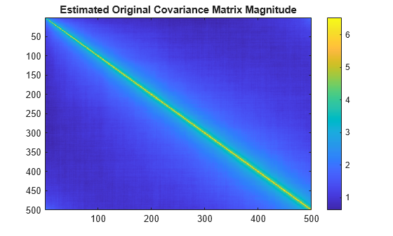

Figure contains an axes object. The axes object with title Estimated Original Covariance Matrix Magnitude contains an object of type image.

Apply the whitening transformation.

R = cov(sig');
W = whiteningmat(R);
sigwhite = W*sig;
covMatrixWhiten = cov(sigwhite');

Display the whitened covariance matrix.

figure
imagesc(abs(covMatrixWhiten))
colorbar;
title("Estimated Whitened Covariance Matrix Magnitude")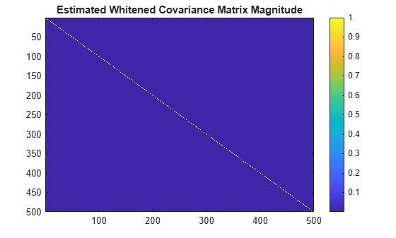

Figure contains an axes object. The axes object with title Estimated Whitened Covariance Matrix Magnitude contains an object of type image.

Perform LRT Detection under Colored Gaussian Noise

Open Live Script

Generate M=1000 independent realizations of data contaminated by colored noise of dimension N=10. Apply whitening to the data before LRT detection to maintain a constant probability of false alarm. Display the probability of false alarm under the null hypothesis and the probability of detection under the alternative hypothesis.

rng default
lrt = phased.LRTDetector(DataComplexity="Complex", ...
    ProbabilityFalseAlarm=0.1);

Create colored Gaussian noise.

N = 10;
M = 1000;
A = 10*rand(N);
R_noise = A'*A;
L_noise = chol(R_noise/2,"lower");

Create the whitening matrix.

noisevar = 1;
w = whiteningmat(R_noise,OutputNoisePower=noisevar);

Whiten the known reference signal.

xref = 5*ones(N,1);
xref_whiten = w*xref;

Perform LRT detection under a null hypothesis.

x0 = L_noise*(randn(N,M) + 1i*randn(N,M));
x0_whiten = w*x0;
dresult0 = lrt(x0_whiten,xref_whiten,noisevar);

Compute the probability of false alarm.

Pfa_whiten = sum(dresult0)/M;
display(Pfa_whiten)

Pfa_whiten = 
0.1030

Perform LRT detection under an alternative hypothesis

x1 = xref + L_noise*(randn(N,M) + 1i*randn(N,M));
x1_whiten = w*x1;
dresult1 = lrt(x1_whiten,xref_whiten,noisevar);

Compute the probability of detection.

Pd_whiten = sum(dresult1)/M;
display(Pd_whiten)

Pd_whiten = 
0.6670

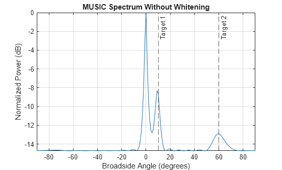
Perform MUSIC Estimation under Clutter

Open Live Script

Consider two target signals impinging on a ULA of N=16 elements. The ULA also receives correlated clutter over different elements. Assume the covariance of clutter-plus-noise covariance matrix is known. Plot the MUSIC estimation result without applying whitening and plot the MUSIC estimation result after applying whitening.

rng default
fc = 150.0e6;
N = 16;
array = phased.ULA(NumElements=N,ElementSpacing=1.0);
estimator = phased.MUSICEstimator(SensorArray=array,...
    OperatingFrequency=fc,NumSignals=2, ...
    DOAOutputPort=true,NumSignalsSource="Property");

Generate the received signals.

fs = 8000;
t = (0:1/fs:1).';
sig1 = cos(2*pi*t*300.0);
sig2 = cos(2*pi*t*400.0);
az_true = [10, 60];
el_true = [20 -5];
sig = collectPlaneWave(array,[sig1 sig2], ...
    [az_true; el_true],fc);

Generate received clutter-plus-noise realizations.

corr_coeff = 0.9;
ula_indices = 0:N-1;
R = corr_coeff.^ abs(ula_indices - ula_indices');
U = chol(R/2,"upper");
clutter = (randn(size(sig)) + 1i*randn(size(sig)))*U;

Perform MUSIC estimation before whitening.

[y,az_no_whiten] = estimator(sig + clutter);
az_no_whiten = broadside2az(sort(az_no_whiten),[20 -5])

az_no_whiten = 1×2

         0    9.0347

figure
plotSpectrum(estimator,"NormalizeResponse",true)
title("MUSIC Spectrum Without Whitening")
tgtlabel = {"Target 1","Target 2"};
xline(az_true,"--",tgtlabel)

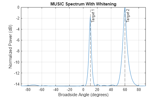
Figure contains an axes object. The axes object with title MUSIC Spectrum Without Whitening, xlabel Broadside Angle (degrees), ylabel Normalized Power (dB) contains 3 objects of type line, constantline. This object represents 1 GHz.

Perform MUSIC estimation after whitening.

w = whiteningmat(R);
data_whiten = (sig + clutter)*w.';
[y_whiten,az_whiten] = estimator(data_whiten);
az_whiten = broadside2az(sort(az_whiten),[20 -5])

az_whiten = 1×2

   10.6490   60.3813

figure
plotSpectrum(estimator,"NormalizeResponse",true)
title("MUSIC Spectrum With Whitening")
xline(az_true,"--",tgtlabel)

Figure contains an axes object. The axes object with title MUSIC Spectrum With Whitening, xlabel Broadside Angle (degrees), ylabel Normalized Power (dB) contains 3 objects of type line, constantline. This object represents 1 GHz.

Target Angle Detection with Interference Mitigation

Open Live Script

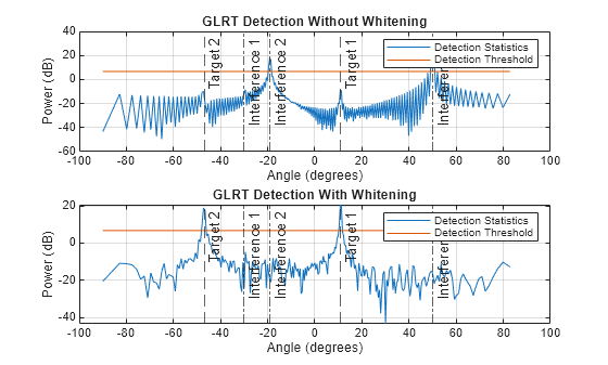
Consider two target signals impinging on a ULA of N=128 elements. The ULA also receives three interference signals. Assume the covariance of interference-plus-noise covariance matrix is known. Plot GLRT detection result without applying whitening and GLRT detection result with whitening applied before angle detection.

rng default
glrt = phased.GLRTDetector(DataComplexity = "Complex", ...
    ProbabilityFalseAlarm = 0.01, ...
    ThresholdOutputPort = true);

Create two targets located at 11 and -47 degrees in azimuth.

tarAng = [11,-47];
tarNum = length(tarAng);

Create a ULA with 128 elements and half-wavelength element spacing.

N = 128;
fc = 3e8;
elementPos = (0:N-1)*physconst("LightSpeed")/fc/2;

Create single-snapshot received signal from two targets at the ULA.

tarAmp = 1/sqrt(2)*(randn(tarNum,1)+1i*randn(tarNum,1));
signal = steervec(elementPos,tarAng)*tarAmp;

Create three interference sources located at -30, -19 and 50 degrees.

intAng = [-30,-19,50]; 
intNum = length(intAng);

Create single-snapshot complex colored Gaussian noise at the ULA.

npow = 0.1;
intAmp = 10/sqrt(2)*(randn(intNum,1)+1i*randn(intNum,1));
Aint= steervec(elementPos,intAng);
Rint = Aint*diag((abs(intAmp)).^2)*Aint';
Rint = (Rint+Rint')/2;
R = npow*eye(N) + Rint;
noise = chol(R/2,"lower")*(randn(N,1)+1i*randn(N,1));
x = signal + noise;

Divide angle space into 256 angle bins.

D = 256;
angGrid = asind(2*(-D/2:D/2-1)/D);

Perform GLRT detection without whitening.

obs = permute(steervec(elementPos,angGrid),[1 3 2]);
hyp = [1,0]; [~,stat,th] = glrt(x,hyp,obs);

Perform GLRT detection with whitening.

w = whiteningmat(R);
x_whiten = w*x;
svs = w*steervec(elementPos,angGrid);
obs_whiten = permute(svs,[1 3 2]);
[~,stat_whiten,th_whiten] = glrt(x_whiten,hyp,obs_whiten);

Plot GLRT detection statistics at the 256 angle bins.

figure
ax1 = subplot(2,1,1);
plot(angGrid,pow2db(stat))
hold on
grid on
plot(angGrid,pow2db(th*ones(1,D)))
title(ax1,"GLRT Detection Without Whitening")
ax2 = subplot(2,1,2);
plot(angGrid,pow2db(stat_whiten))
hold on
grid on
plot(angGrid,pow2db(th_whiten*ones(1,D)))
title(ax2,"GLRT Detection With Whitening")
ax = {ax1,ax2};
for idx = 1:2
    xlabel(ax{idx},"Angle (degrees)")
    ylabel(ax{idx},"Power (dB)")
    tgtlabel = {"Target 1","Target 2"};
    xline(ax{idx},tarAng,"--",tgtlabel)
    intlabel = {"Interference 1", ...
        "Interference 2","Interference 3"};
    xline(ax{idx},intAng,"-.",intlabel)
    legend(ax{idx},{"Detection Statistics", ...
        "Detection Threshold"})
end

Input Arguments

collapse all

`Ncov` — Noise covariance
N-by-N real-valued positive definite matrix | N-by-N complex-valued positive definite matrix

Noise covariance, specified as an N-by-N real-valued positive definite matrix or N-by-N complex-valued positive definite matrix.

Data Types: single | double
Complex Number Support: Yes

`pow` — Output whitened noise power
1 (default) | positive scalar

Output power of whitened noise, specified as a positive real scalar.

Example: 10.0

Data Types: single | double

Output Arguments

collapse all

`W` — Whitening transformation matrix
N-by-N real-valued positive definite matrix | N-by-N complex-valued positive definite matrix

Whitening transformation matrix, returned as an N-by-N real-valued positive definite matrix or an N-by-N complex-valued positive definite matrix. The complexity of W matches the complexity of ncov.

Data Types: single | double
Complex Number Support: Yes

Algorithms

collapse all

Data Whitening

This function uses Cholesky decomposition to whiten the covariance matrix Ncov into a scaled identity matrix. See [1] or [2]. When applied to a signal in noise it can be used to generate a transformed signal in white noise. Start with the data model x = s + z, where x is a noise-free deterministic signal and z is zero-mean Gaussian noise specified by the covariance matrix R_n. You can input the noise covariance matrix using the ncov argument. Applying a whitening matrix, W to the data x, produces a transformed signal embedded in white noise.

$x^{'} = W x = W s + W z$

The covariance of the whitened noise, represented as $W z$ , is given by

$W n_{cov} W' = P 1_{N}$

where P is the white noise power specified by the pow input argument. N represents the dimensions of the noise matrix. When pow equals one, the whitened noise covariance matrix is the identity matrix. For other positive values of pow the whitened data covariance matrix is a scaled version of the identity matrix.

The images below show the magnitudes of the original unwhitened covariance matrix and the whitened covariance matrix.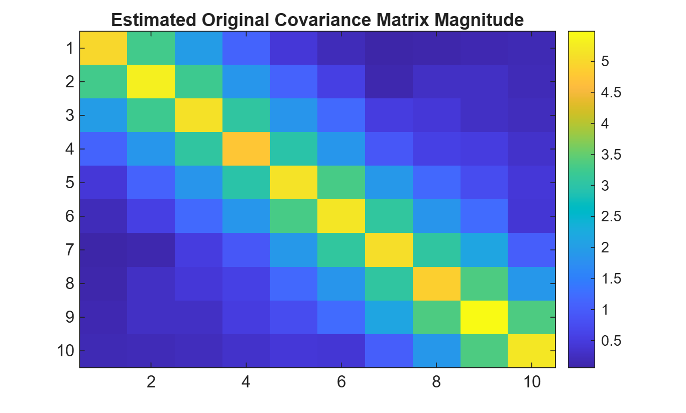 Original Unwhitened Noise Covariance Matrix Whitend Noise Covariance Matrix

Data precision

This function supports single and double precision for input arguments. If the input argument ncov is single precision, the outputs are single precision. If the input argument ncov is double precision, the outputs are double precision. The precision of the outputs are independent of the precision of the other arguments.

References

[1] Steven M. Kay, Fundamentals of Statistical Signal Processing, Detection Theory, 1998.

[2] Golub, Gene H. and Van Loan, Charles F. Matrix Computations - 4th Edition}, Philadelphia, PA: Johns Hopkins University Press, 2013.

Version History

Introduced in R2026a

whiteningmat

Syntax

Description

Examples

Plot Whitened Covariance Matrix

Plot Whitened Complex Covariance Matrix

Perform LRT Detection under Colored Gaussian Noise

Perform MUSIC Estimation under Clutter

Target Angle Detection with Interference Mitigation

Input Arguments

Ncov — Noise covariance N-by-N real-valued positive definite matrix | N-by-N complex-valued positive definite matrix

pow — Output whitened noise power 1 (default) | positive scalar

Output Arguments

W — Whitening transformation matrix N-by-N real-valued positive definite matrix | N-by-N complex-valued positive definite matrix

Algorithms

Data Whitening

Data precision

References

Version History

See Also

`Ncov` — Noise covariance
N-by-N real-valued positive definite matrix | N-by-N complex-valued positive definite matrix

`pow` — Output whitened noise power
1 (default) | positive scalar

`W` — Whitening transformation matrix
N-by-N real-valued positive definite matrix | N-by-N complex-valued positive definite matrix