Benefits of Adaptive Beamforming

Narrowband Phase Shift Beamformer for a ULA uses weights chosen independent of any data received by the array. The weights in the narrowband phase shift beamformer steer the array response in a specified direction. However, they do not account for any interference scenarios. As a result, these conventional beamformers are susceptible to interference signals. Such interference signals can be a particular problem if they occur at sidelobes of the array response.

By contrast, adaptive, or statistically optimum, beamformers can account for interference signals. An adaptive beamformer algorithm chooses the weights based on the statistics of the received data. For example, an adaptive beamformer can improve the SNR by using the received data to place nulls in the array response. These nulls are placed at angles corresponding to the interference signals.

Support for Adaptive Beamforming

Phased Array System Toolbox™ software provides these adaptive beamformers:

Nulling with LCMV Beamformer

This example shows how to use an LCMV beamformer to point a null of the array response in the direction of an interfering source. The array is a 10-element uniform linear array (ULA). By default, the ULA elements are isotropic antennas created by the phased.IsotropicAntennaElement System object™. Set the frequency range of the antenna elements so that the carrier frequency lies within the operating range. The carrier frequency is 1 GHz.

fc = 1e9;
lambda = physconst('LightSpeed')/fc;
array = phased.ULA('NumElements',10,'ElementSpacing',lambda/2);
array.Element.FrequencyRange = [8e8 1.2e9];

Simulate a test signal using a simple rectangular pulse.

t = linspace(0,0.3,300)';
testsig = zeros(size(t));
testsig(201:205) = 1;

Assume the rectangular pulse is incident on the ULA from an angle of 30° azimuth and 0° elevation. Use the collectPlaneWave function of the ULA System object to simulate reception of the pulse waveform from the incident angle.

angle_of_arrival = [30;0];
x = collectPlaneWave(array,testsig,angle_of_arrival,fc);

The signal x is a matrix with ten columns. Each column represents the received signal at one of the array elements.

Construct a conventional phase-shift beamformer. Set the WeightsOutputPort property to true to output the spatial filter weights.

convbeamformer = phased.PhaseShiftBeamformer('SensorArray',array,...
    'OperatingFrequency',1e9,'Direction',angle_of_arrival,...
    'WeightsOutputPort',true);

Add complex-valued white Gaussian noise to the signal x. Set the default random number stream for reproducible results.

rng default
npower = 0.5;
x = x + sqrt(npower/2)*(randn(size(x)) + 1i*randn(size(x)));

Create a 10W interference source. Specify the barrage jammer to have an effective radiated power of 10 W. The interference signal from the barrage jammer is incident on the ULA from an angle of 120° azimuth and 0° elevation. Use the collectPlaneWave function of the ULA System object to simulate reception of the jammer signal.

jamsig = sqrt(10)*randn(300,1);
jammer_angle = [120;0];
jamsig = collectPlaneWave(array,jamsig,jammer_angle,fc);

Add complex-valued white Gaussian noise to simulate noise contributions not directly associated with the jamming signal. Again, set the default random number stream for reproducible results. This noise power is 0 dB below the jammer power. Beamform the signal using a conventional beamformer.

noisePwr = 1e-5;
rng(2008);
noise = sqrt(noisePwr/2)*...
    (randn(size(jamsig)) + 1j*randn(size(jamsig)));
jamsig = jamsig + noise;
rxsig = x + jamsig;
[yout,w] = convbeamformer(rxsig);

Implement the adaptive LCMV beamformer using the same ULA array. Use the target-free data, jamsig, as training data. Output the beamformed signal and the beamformer weights.

steeringvector = phased.SteeringVector('SensorArray',array,...
    'PropagationSpeed',physconst('LightSpeed'));
LCMVbeamformer = phased.LCMVBeamformer('DesiredResponse',1,...
    'TrainingInputPort',true,'WeightsOutputPort',true);
LCMVbeamformer.Constraint = steeringvector(fc,angle_of_arrival);
LCMVbeamformer.DesiredResponse = 1;
[yLCMV,wLCMV] = LCMVbeamformer(rxsig,jamsig);

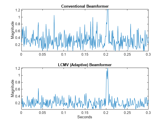
Plot the conventional beamformer output and the adaptive beamformer output.

subplot(211)
plot(t,abs(yout))
axis tight
title('Conventional Beamformer')
ylabel('Magnitude')
subplot(212)
plot(t,abs(yLCMV))
axis tight
title('LCMV (Adaptive) Beamformer')
xlabel('Seconds')
ylabel('Magnitude')

The adaptive beamformer significantly improves the SNR of the rectangular pulse at 0.2 s.

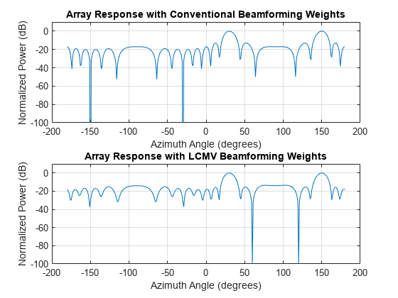
Using conventional and LCMV weights, plot the responses for each beamformer.

subplot(211)
pattern(array,fc,[-180:180],0,'PropagationSpeed',physconst('LightSpeed'),...
    'CoordinateSystem','rectangular','Type','powerdb','Normalize',true,...
    'Weights',w)
title('Array Response with Conventional Beamforming Weights');
subplot(212)
pattern(array,fc,[-180:180],0,'PropagationSpeed',physconst('LightSpeed'),...)
    'CoordinateSystem','rectangular','Type','powerdb','Normalize',true,...
    'Weights',wLCMV)
title('Array Response with LCMV Beamforming Weights');

The adaptive beamform places a null at the arrival angle of the interference signal, 120°.