Conventional Beamforming

Uses for Beamformers

You can use a beamformer to spatially filter the arriving signals. Accentuating or attenuating signals that arrive from specific directions helps you distinguish between signals of interest and interfering signals from other directions.

Support for Conventional Beamforming

You can implement a narrowband phase shift beamformer using phased.PhaseShiftBeamformer. When you use this object, you must specify these aspects of the situation you are simulating:

Sensor array
Signal propagation speed
System operating frequency
Beamforming direction

For wideband beamformers, see Wideband Beamforming.

Narrowband Phase Shift Beamformer for a ULA

Open Script

This example shows how to create and beamform a 10-element ULA. Assume the carrier frequency is 1 GHz. Set the array element spacing to be one-half the carrier wavelength.

fc = 1e9;
lambda = physconst('LightSpeed')/fc;
array = phased.ULA('NumElements',10,'ElementSpacing',lambda/2);

By default, the ULA elements are isotropic antennas created by the phased.IsotropicAntennaElement System object™. Set the frequency range of the antenna elements so that the carrier frequency lies within the operating range.

array.Element.FrequencyRange = [8e8 1.2e9];

Simulate a test signal. For this example, use a simple rectangular pulse.

t = linspace(0,0.3,300)';
testsig = zeros(size(t));
testsig(201:205) = 1;

Assume the rectangular pulse is incident on the ULA from an angle of 30° azimuth and 0° elevation. Use the collectPlaneWave function of the ULA System object to simulate reception of the pulse waveform from the specified angle.

angle_of_arrival = [30;0];
x = collectPlaneWave(array,testsig,angle_of_arrival,fc);

The signal |x| is a matrix with ten columns. Each column represents the received signal at one of the array elements.

Add complex-valued Gaussian noise to the signal |x|. Reset the default random number stream for reproducible results. Plot the magnitudes of the received pulses at the first four elements of the ULA.

rng default
npower = 0.5;
x = x + sqrt(npower/2)*(randn(size(x)) + 1i*randn(size(x)));
subplot(221)
plot(t,abs(x(:,1)))
title('Element 1 (magnitude)')
axis tight
ylabel('Magnitude')
subplot(222)
plot(t,abs(x(:,2)))
title('Element 2 (magnitude)')
axis tight
ylabel('Magnitude')
subplot(223)
plot(t,abs(x(:,3)))
title('Element 3 (magnitude)')
axis tight
xlabel('Seconds')
ylabel('Magnitude')
subplot(224)
plot(t,abs(x(:,4)))
title('Element 4 (magnitude)')
axis tight
xlabel('Seconds')
ylabel('Magnitude')

Construct a phase-shift beamformer. Set the WeightsOutputPort property to true to output the spatial filter weights that point the beamformer to the angle of arrival.

beamformer = phased.PhaseShiftBeamformer('SensorArray',array, ...
    'OperatingFrequency',1e9,'Direction',angle_of_arrival, ...
    'WeightsOutputPort',true);

Execute the phase shift beamformer to compute the beamformer output and to compute the applied weights.

[y,w] = beamformer(x);

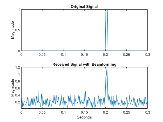
Plot the magnitude of the output waveform along with the noise-free original waveform for comparison.

subplot(211)
plot(t,abs(testsig))
axis tight
title('Original Signal')
ylabel('Magnitude')
subplot(212)
plot(t,abs(y))
axis tight
title('Received Signal with Beamforming')
ylabel('Magnitude')
xlabel('Seconds')

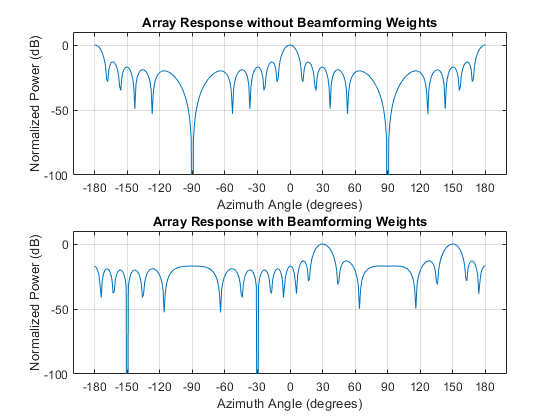
To examine the effect of beamforming weights on the array response, plot the array normalized power response with and without beamforming weights.

azang = -180:30:180;
subplot(211)
pattern(array,fc,[-180:180],0,'CoordinateSystem','rectangular',...
    'Type','powerdb','PropagationSpeed',physconst('LightSpeed'))
xticks(azang)
set(gca,'Fontsize',9)
title('Array Response without Beamforming Weights')
subplot(212)

pattern(array,fc,[-180:180],0,'CoordinateSystem','rectangular',...
    'Type','powerdb','PropagationSpeed',physconst('LightSpeed'),...
    'Weights',w)
xticks(azang)
set(gca,'Fontsize',9)
title('Array Response with Beamforming Weights')