Array Pattern Synthesis Part III: Deep Learning

This example uses:

This example shows how to design and train a convolutional neural network (CNN) to compute the element weights that produce a desired pattern.

Introduction

Pattern synthesis is an important topic in array processing. Array weights help shape the beam pattern of a sensor array to match a desired pattern. Traditionally, pattern synthesis algorithms are often borrowed from filter design techniques due to the similarity between the spatial signal processing and frequency domain signal processing. Many such algorithms are covered in our Array Pattern Synthesis Part I example. Unfortunately, those algorithms are often not very flexible to accommodate different kinds of constraints. Therefore, as a more general solution, various optimization techniques are used to produce desired patterns. Some frequently used optimization solvers are introduced in the Array Pattern Synthesis Part II example. Although the optimization-based algorithms are very flexible, for large arrays, it takes a while to converge into the optimal solution. This pitfall makes it difficult to form a given beam pattern in real time.

Deep learning techniques have seen many successes in computer vision and natural language processing. Although a deep learning network needs to be trained off line; once trained, the resulting network can be used to achieve real time performance. Hence, a deep learning network may be able to provide a solution for real time pattern synthesis, as suggested in [1].

Array Definition

Consider a circular planar array with a radius of 3 meters. The elements are located on a rectangular grid with an element spacing of 0.5 meters.

r = 3;
delta = 0.5;
lambda = 1;
[pos,N] = getCircularPlanarArrayPositions(r,delta,lambda);

The array aperture looks like below. The array is in the y-z plane with broadside aligned with x axis.

ant = phased.ConformalArray('ElementPosition',pos);
viewArray(ant,'title','Circular Planar Array Aperture')

Pattern Synthesis with Optimization

As explained in the Array Pattern Synthesis Part II example, optimization techniques can be used to derive the pattern synthesis weights. Assume we would like to have a pattern whose main lobe is along azimuth and elevation 0 degrees. The pattern should also satisfy the following constraints:

Maximize the directivity
Suppress interferences 30 dB below mainlobe
Keep sidelobe levels within -20 and 20 degrees azimuth or elevation be 17 dB below mainlobe

% define main lobe direction
ang_d = [0;0];

% define interference directions and corresponding desired response
ang_i = [12 10;13 10];
r_i = [-30 -30]; 

% define the region where sidelobe levels below desired level
ang_c_az_grid = [-20:0.5:-10 10:0.5:20]+ang_d(1); 
ang_c_el_grid = [-20:0.5:-10 10:0.5:20]+ang_d(2); 
[ang_c_az,ang_c_el] = meshgrid(ang_c_az_grid,ang_c_el_grid);
ang_c = [ang_c_az(:).';ang_c_el(:).'];
ang_c = setdiff(ang_c.',ang_i.','rows').';
r_c_th = -17; 
r_c = r_c_th*ones(1,size(ang_c,2));

With all constraints defined, we can use optimization solver to derived the array weights that can provide us the desired pattern. For details on the optimization solver, please refer to the Array Pattern Synthesis Part II example.

% Compute weights using optimization solvers
tic;
[w_op,Rn] = helperPatternSynthesis(pos,ang_d,[],[],[ang_i,ang_c],[r_i,r_c]);

Optimal solution found.

t = toc;

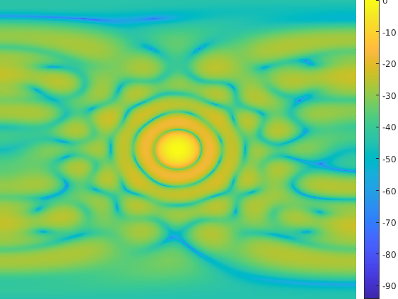
The resulting pattern is displayed below

az_plot = -90:0.25:90;
el_plot = -90:0.25:90;
w = w_op(1:N)+1i*w_op(N+1:2*N);
pat_opt = computePattern(pos,az_plot,el_plot,w);
plotPattern(az_plot,el_plot,pat_opt,'Optimization');

We can measure the quality of this pattern by measuring whether the resulting pattern matches the requirements.

[d,intdb,sllpct] = measurePattern(pat_opt,ang_d,ang_i,ang_c,az_plot,el_plot,r_c_th,Rn,w);
d_max = pow2db(4*pi*N^2/abs(sum(Rn,"all")));
Metrics = ["Directivity (dBi)";"Interference Suppression (dB)";"Sidelobe Over Requirement Percentage"];
Measured = {d;intdb;sllpct};
Requirement = {d_max;r_i;0};
metrictab = table(Metrics,Measured,Requirement)

metrictab=3×3 table
                   Metrics                          Measured           Requirement
    ______________________________________    _____________________    ___________

    "Directivity (dBi)"                       {[          22.2814]}    {[22.1824]}
    "Interference Suppression (dB)"           {[-29.3262 -30.6321]}    {[-30 -30]}
    "Sidelobe Over Requirement Percentage"    {[                0]}    {[      0]}

We can see that the resulting metrics are very good. However, it does take some time to calculate the weights.

fprintf('Weights computation time: %f seconds.\n',t);

Weights computation time: 28.869624 seconds.

Deep Learning Network

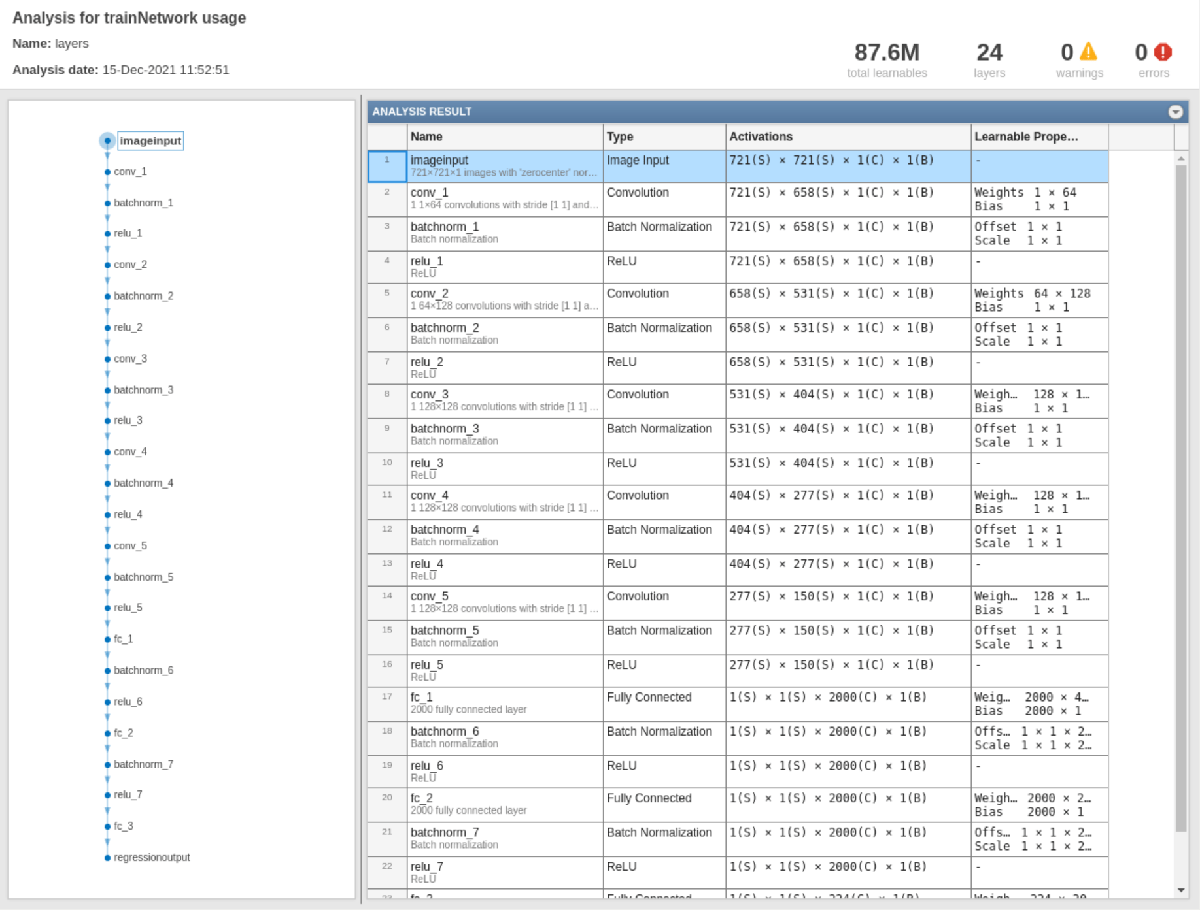
To perform pattern synthesis using deep learning, we create a convolution neural network (CNN) as outlined in [1]. A beam pattern is defined over a range of azimuth and elevation angles. Therefore, the pattern can be represented as an image and our input layer take the image as the input. The output is the weights that produces such a pattern.

layers = [
imageInputLayer([721 721 1],'Normalization','zerocenter')

convolution2dLayer([1,64],1)
batchNormalizationLayer
reluLayer

convolution2dLayer([64,128],1)
batchNormalizationLayer
reluLayer

convolution2dLayer([128,128],1)
batchNormalizationLayer
reluLayer

convolution2dLayer([128,128],1)
batchNormalizationLayer
reluLayer

convolution2dLayer([128,128],1)
batchNormalizationLayer
reluLayer

fullyConnectedLayer(2000)
batchNormalizationLayer
reluLayer

fullyConnectedLayer(2000)
batchNormalizationLayer
reluLayer

fullyConnectedLayer(224)
];

analyzeNetwork(layers);

Training and Testing Data Synthesis

To train and test the network, we can generate patterns with random mainlobe and interference placements. We will derive the optimal weights via optimization solver and then use the derived pattern as the input to compute the weights through network and hope that the resulting weights will match the optimal weights.

dataURL = 'https://ssd.mathworks.com/supportfiles/phased/data/ArraySynthesisDLData.zip';
saveFolder = tempdir; 
dataDir = 'datasetSmallE';
zipFile = fullfile(saveFolder,'ArraySynthesisDLData.zip');
if ~exist(zipFile,'file')
    websave(zipFile,dataURL);
    % Unzip the data
    unzip(zipFile,tempdir)
end

signalDs = signalDatastore(fullfile(saveFolder,dataDir),"ReadFcn",@readTrainAndValFile);
signalDs = shuffle(signalDs);

Split the dataset into training and validation set

[trainInd,valInd,testInd] = dividerand(1:numel(signalDs.Files),0.8,0.1,0.1);
trainDs = subset(signalDs,trainInd);
validDs = subset(signalDs,valInd);
testDs = subset(signalDs,testInd);
testDs.ReadFcn = @readTestFile;
% Number of files used for training, validation and testing
fprintf('Number of training, validating, and testing data are %d, %d, and %d, respectively.',...
    numel(trainDs.Files),numel(validDs.Files),numel(testDs.Files));

Number of training, validating, and testing data are 778, 97, and 97, respectively.

Train Network

Now we can train the network

trainNetworkNow = false;
if trainNetworkNow
    options = trainingOptions('adam', ...
        'MaxEpochs',30,...
        'GradientDecayFactor', 0.9,...
        'SquaredGradientDecayFactor',0.999,...
        'InitialLearnRate',1e-3, ...
        'Verbose',false, ...
        'Plots','training-progress',...
        'LearnRateSchedule','none',...
        'ValidationData',validDs,...
        'ValidationFrequency',3,...
        'Metric','rmse'); %#ok<UNRCH> 
    net = trainnet(trainDs,layers,'mse',options);
else
    load(fullfile(saveFolder,'helperPatternSynthesisDL.mat'),'net');
end

Test Trained Network

Use the pattern derived in the early section, let us see if the trained network can provide a sastifying pattern

tic;
w_dl = double(minibatchpredict(net, cast(pat_opt,'int8')))';
t_dl = toc;
w = w_dl(1:N)+1i*w_dl(N+1:2*N);
w = w./norm(arrayfactor(pos,ang_d,w));
pat_dl = computePattern(pos,az_plot,el_plot,w);
plotPattern(az_plot,el_plot,pat_dl,'Deep Learning');

[d,intdb,sllpct] = measurePattern(pat_dl,ang_d,ang_i,ang_c,az_plot,el_plot,r_c_th,Rn,w);
d_max = pow2db(4*pi*N^2/abs(sum(Rn,"all")));
Metrics = ["Directivity (dBi)";"Interference Suppression (dB)";"Sidelobe Over Requirement Percentage"];
Measured = {d;intdb;sllpct};
Requirement = {d_max;r_i;0};
metrictab = table(Metrics,Measured,Requirement)

metrictab=3×3 table
                   Metrics                          Measured           Requirement
    ______________________________________    _____________________    ___________

    "Directivity (dBi)"                       {[          22.0606]}    {[22.1824]}
    "Interference Suppression (dB)"           {[-21.6913 -21.9344]}    {[-30 -30]}
    "Sidelobe Over Requirement Percentage"    {[                0]}    {[      0]}

fprintf('Weights computation time: %f seconds.\n',t_dl);

Weights computation time: 10.487740 seconds.

We can see that the predicted pattern gives good result in terms of directivity and sidelobe suppression. It is not as good as achieving the interference suppression. We may be able to improve this with more training data.

Conclusion

This example shows how to create and train a CNN to perform pattern synthesis for a given array. Although the deep learning network can generate pattern synthesis weights much faster, it has its own drawbacks. For example, the network requires a large amount of data to train. In addition, the network is specific to a specific array geometry. Therefore, if the array formation changes, the network needs to be retrained.

References

[1] Bianco, Simone, Maurizio Feo, Paolo Napoletano, Giovanni Petraglia, Alberto Raimondi, and Pietro Vinetti. "AESA Adaptive Beamforming Using Deep Learning." Proceedings of 2020 IEEE Radar Conference, 2020.

Support Files

Define Array

function [pos,N] = getCircularPlanarArrayPositions(radius,delta,lambda)
    n = round(radius/delta*2);
    htemp = phased.URA(n, delta, ...
        'Lattice', 'Rectangular');
    pos = getElementPosition(htemp)/lambda;
    elemToRemove = sum(pos.^2)>radius^2;
    pos(:,elemToRemove) = [];
    N = size(pos,2);
end

Compute Pattern

function pat = computePattern(pos,az_plot,el_plot,w)
    pat = zeros(numel(el_plot),numel(az_plot));
    for m = 1:numel(el_plot)
        pat(m,:) = mag2db(abs(arrayfactor(pos,[az_plot;el_plot(m)*ones(size(az_plot))],w)));
    end
end

Plot Pattern

function plotPattern(az_plot,el_plot,pat,algstr)
    surf(az_plot,el_plot,pat,'EdgeColor','none');
    colorbar;
    view(0,90);
    xlabel('Azimuth (deg)');
    ylabel('Elevation (deg)');
    title(sprintf('Beam Pattern via %s',algstr));
    axis tight
end

Measure Pattern Metrics

function [d,intdb,sllpct] = measurePattern(pat,ang_d,ang_i,ang_c,az_plot,el_plot,sllbar,Rn,w)
az_step = mean(diff(az_plot));
el_step = mean(diff(el_plot));
d = pat(sub2ind(size(pat),(ang_d(1)-az_plot(1))/az_step+1,(ang_d(2)-el_plot(1))/el_step+1))+...
    pow2db(4*pi)-pow2db(abs(w'*Rn*w));
intdb = pat(sub2ind(size(pat),(ang_i(1,:)-az_plot(1))/az_step+1,(ang_i(2,:)-el_plot(1))/el_step+1))-max(pat,[],'all');
slldb = pat(sub2ind(size(pat),(ang_c(1,:)-az_plot(1))/az_step+1,(ang_c(2,:)-el_plot(1))/el_step+1))-max(pat,[],'all');
sllpct = sum(slldb>sllbar)/numel(slldb);
end

Read Data Files

function dataOut = readTrainAndValFile(filename)
  
    data = struct2cell(load(filename));
    data = data{1};

    dataOut{1} = data{1};
    dataOut{2} = normalize(data{2})';
end


function dataOut = readTestFile(filename)
  
    data = struct2cell(load(filename));
    data = data{1};
    dataOut = data;
end