Deep Underwater Channel Target Detection Using Active Sonar

R2026b

Since R2026b

This example uses:

This example demonstrates an active monostatic sonar scenario using the bellhopModel object for underwater acoustic propagation. The example simulates an underwater acoustic propagation channel between:

Transmitter → Target (forward propagation)
Target → Receiver (return propagation)

The key advantage of the Bellhop beam tracing model is its ability to model ray refraction through a depth-dependent sound speed profile. Sound speed varies with depth because of changes in temperature and pressure. This variation causes acoustic rays to bend and produces convergence zones, shadow zones, and depth-dependent arrival angles. For an example of underwater target detection in a shallow underwater channel with constant sound speed, see Underwater Target Detection with an Active Sonar System.

Prerequisites

The bellhopModel object requires you to set the path to the Bellhop executable in MATLAB® the first time you use the object. The bellhopConfiguration function manages the path. If the executable path is not already set, set setExecutablePath to true and select the executable path.

setExecutablePath = false;
if setExecutablePath
    executablePath = "C:\Users\Username\bellhopEXE\bellhop.exe"; %#ok
    bellhopConfiguration(ExecutablePath=executablePath);
end

Environment and Geometry

Configure a deep-ocean environment at the Bermuda Rise. A sound speed profile computed from World Ocean Atlas (WOA) 2023 temperature [2,3] and salinity [2,4] data produces a sound channel axis near 1250 m depth. Place the sonar transceiver at 1000 m, near the sound fixing and ranging (SOFAR) axis. Then, place a target at 50 km range, 800 m depth. The 50 km range places the target in the first convergence zone, where refracted rays focus and transmission loss is significantly lower than what spherical spreading predicts.

fc = 1000;
c = 1500;

srcPos = [0; 0; 1000];
tgtPos = [0; 50000; 800];
rxPos = srcPos;

Create the bellhopModel object and use a $\pm$ 15 degree ray fan to capture the near-axial refracted paths that form the SOFAR channel.

bh = bellhopModel();
bh.RayElevationAngles = [-15 15];

Bathymetry

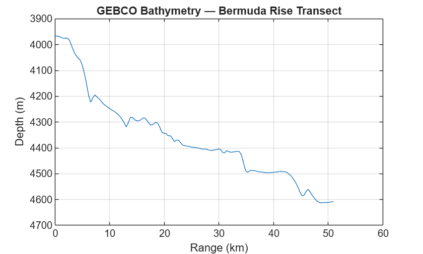
Load ocean bathymetry from the gebcoBermudaRise.nc file [5], a General Bathymetric Chart of the Oceans (GEBCO) 2026 subset covering the Bermuda Rise in the North Atlantic. The gebcoBermudaRise.nc file includes data for longitudes between -64.5479 and -63.9229 degrees E and latitudes between 31.9521and 32.0479 degrees N. The helperBathymetry function reads the NetCDF file and extracts a depth profile along the source-to-target transect. The geographic coordinates define an East-West track at 32 degrees N.

srcLat = 32.0; 
srcLon = -64.5;
rxLat = 32.0;  
rxLon = -63.96;
bathymetry = helperBathymetry("gebcoBermudaRise.nc",srcLat, ...
    srcLon,rxLat,rxLon);
bh.BottomBathymetryProfile = bathymetry;

Visualize the bathymetry transect.

plot(bathymetry(:,1)/1000, bathymetry(:,2))
set(gca,YDir="reverse")
xlabel("Range (km)")
ylabel("Depth (m)")
title("GEBCO Bathymetry — Bermuda Rise Transect")
grid on

Figure contains an axes object. The axes object with title GEBCO Bathymetry — Bermuda Rise Transect, xlabel Range (km), ylabel Depth (m) contains an object of type line.

Sound Speed Profile

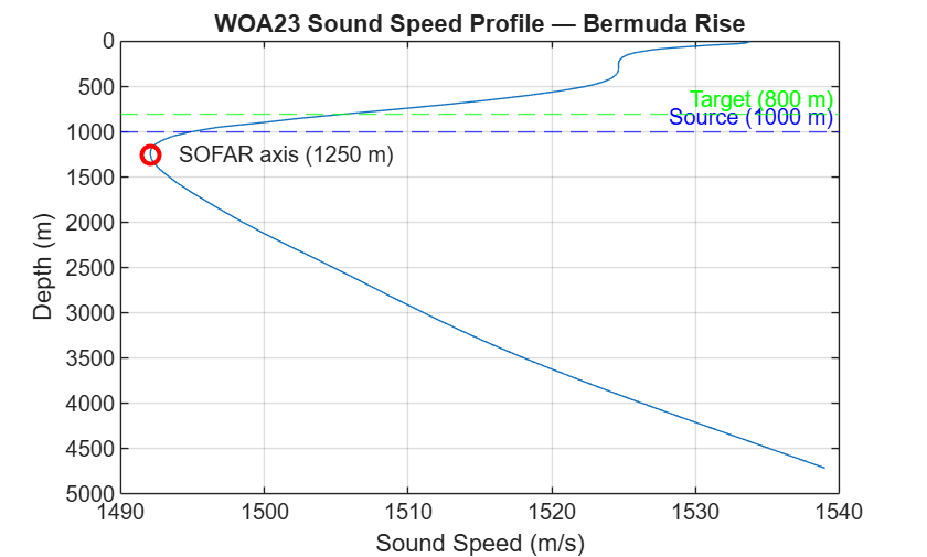
Compute a sound speed profile from WOA 2023 temperature and salinity data using the Mackenzie equation. The helperSoundSpeedProfile function extracts temperature and salinity profiles at the nearest grid point to the source location, and underwaterSoundSpeed converts them to sound speed as a function of depth. The resulting profile captures the real SOFAR channel structure at the Bermuda Rise.

The example includes two NetCDF files, woa23TemperatureBermuda.nc and woa23SalinityBermuda.nc, which contain regional subsets of WOA 2023 temperature and salinity data. The files contain the statistical mean of monthly temperature and salinity on a 1/4° grid for all decades for the month of January. They include data for longitudes between –65.1250 and –64.1250 degrees E, latitudes between 31.3750 and 32.3750 degrees N, and depths between 0 and 5500 m.

[temp, sal, depthWOA] = helperSoundSpeedProfile("woa23TemperatureBermuda.nc", ...
    "woa23SalinityBermuda.nc", srcLat, srcLon);
soundSpeed = underwaterSoundSpeed(temp, sal, depthWOA);

The Bellhop model requires sound speed to be defined at the maximum depth of the bathymetry profile. Verify that the sound speed profile computed from the WOA temperature and salinity data extends to the maximum depth of the Bermuda rise bathymetry. Extrapolate the sound speed if needed.

maxBathyDepth = max(bathymetry(:,2));
if depthWOA(end) < maxBathyDepth
    gradient = (soundSpeed(end) - soundSpeed(end-1)) / (depthWOA(end) - depthWOA(end-1));
    extDepth = maxBathyDepth + 100;
    extSpeed = soundSpeed(end) + gradient * (extDepth - depthWOA(end));
    depthWOA = [depthWOA; extDepth];
    soundSpeed = [soundSpeed; extSpeed];
end

bh.SoundSpeed = soundSpeed;
bh.SoundSpeedDepth = depthWOA;

Visualize the sound speed profile. The sound speed minimum near 1250 m defines the SOFAR channel axis, trapping acoustic energy and enabling long-range propagation with low loss.

plot(bh.SoundSpeed, bh.SoundSpeedDepth)
set(gca,YDir="reverse")
xlabel("Sound Speed (m/s)")
ylabel("Depth (m)")
title("WOA23 Sound Speed Profile — Bermuda Rise")
grid on
hold on
[~, iMin] = min(bh.SoundSpeed);
plot(bh.SoundSpeed(iMin), bh.SoundSpeedDepth(iMin), 'ro', MarkerSize=8,LineWidth=2)
text(bh.SoundSpeed(iMin)+2, bh.SoundSpeedDepth(iMin), sprintf('SOFAR axis (%.0f m)', bh.SoundSpeedDepth(iMin)))
yline(srcPos(3), "b--", sprintf("Source (%.0f m)", srcPos(3)))
yline(tgtPos(3), "g--", sprintf("Target (%.0f m)", tgtPos(3)))
hold off

Figure contains an axes object. The axes object with title WOA23 Sound Speed Profile — Bermuda Rise, xlabel Sound Speed (m/s), ylabel Depth (m) contains 5 objects of type line, text, constantline. One or more of the lines displays its values using only markers

Forward Propagation (Transmitter to Target)

Compute eigenrays from the sonar to the target. At 50 km, the refracted rays that cycle through the SOFAR channel converge, producing multiple arrivals with relatively low transmission loss. This convergence zone effect is the primary mechanism for long-range sonar detection in the deep ocean.

propagationPaths(bh, fc, srcPos, tgtPos);

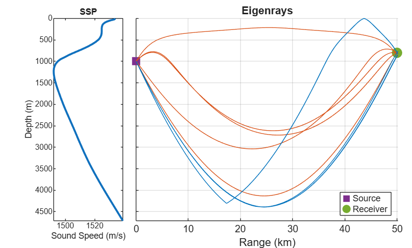
Figure Bellhop Eigenrays contains 2 axes objects. Axes object 1 with title SSP, xlabel Sound Speed (m/s), ylabel Depth (m) contains an object of type line. Axes object 2 with title Eigenrays, xlabel Range (km) contains 16 objects of type line. One or more of the lines displays its values using only markers These objects represent Source, Receiver.

arrivalsForward = propagationPaths(bh, fc, srcPos, tgtPos)

arrivalsForward = 10×7 table
    PathLoss    PathDelay    PhaseShift    AngleOfDeparture    AngleOfArrival    NumSurfaceReflections    NumBottomReflections
    ________    _________    __________    ________________    ______________    _____________________    ____________________

      87.25      33.453            90        0    -7.4466       0    -2.6919               0                       0          
     87.596      33.405             0        0      12.08       0    -9.8881               0                       0          
     88.775      33.454           180        0    -7.0732       0     1.5137               0                       0          
     89.482      33.423            90        0     8.5412       0     5.0977               0                       0          
     98.362      33.533        62.282        0     13.871       0     11.524               1                       1          
     108.38      33.454           180        0    -7.0702       0      1.736               0                       0          
     108.72      33.406       -175.48        0     12.873       0    -10.623               0                       1          
     116.94      32.868            90        0    -11.358       0     10.014               0                       0          
      119.8      33.406       -176.84        0      12.87       0    -11.775               0                       1          
     123.45      33.406       -177.01        0     12.903       0    -11.759               0                       1

Return Propagation (Target to Receiver)

Compute eigenrays from the target back to the receiver. Because the target is at 800 m (above the SOFAR axis at 1000 m), the return paths have different ray geometries.

propagationPaths(bh, fc, tgtPos, rxPos);

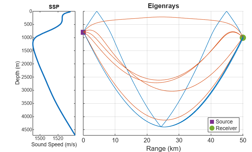
Figure Bellhop Eigenrays contains 2 axes objects. Axes object 1 with title SSP, xlabel Sound Speed (m/s), ylabel Depth (m) contains an object of type line. Axes object 2 with title Eigenrays, xlabel Range (km) contains 17 objects of type line. One or more of the lines displays its values using only markers These objects represent Source, Receiver.

arrivalsReturn = propagationPaths(bh, fc, tgtPos, rxPos)

arrivalsReturn = 8×7 table
    PathLoss    PathDelay    PhaseShift    AngleOfDeparture    AngleOfArrival    NumSurfaceReflections    NumBottomReflections
    ________    _________    __________    ________________    ______________    _____________________    ____________________

     86.503      33.454           180        0    -1.5327       0     7.0648               0                       0          
     87.441      33.453            90        0      2.794       0     7.3432               0                       0          
     87.674      33.405             0        0     9.9358       0    -12.093               0                       0          
     89.751      33.423            90        0    -5.0392       0    -8.5477               0                       0          
      97.99      33.778       -85.951        0    -13.657       0     15.075               2                       1          
        104      33.406       -176.32        0     10.903       0    -12.787               0                       1          
     107.89      33.406       -175.58        0      10.92       0    -12.978               0                       1          
     116.44      32.868            90        0    -9.0384       0     11.143               0                       0

fprintf("Forward: %d refracted, %d bottom-bounce", ...
    sum(arrivalsForward.NumBottomReflections==0), sum(arrivalsForward.NumBottomReflections>0))

Forward: 6 refracted, 4 bottom-bounce

fprintf("Return:  %d refracted, %d bottom-bounce", ...
    sum(arrivalsReturn.NumBottomReflections==0), sum(arrivalsReturn.NumBottomReflections>0))

Return:  5 refracted, 3 bottom-bounce

Waveform and System Parameters

Define a 100 ms Linear FM (chirp) pulse at 1 kHz with 100 Hz sweep bandwidth. The LFM waveform delivers the same energy as a CW pulse of equal duration, but its time-bandwidth product ( $τ β$ = 10) enables pulse compression on receive.

A matched filter compresses the received pulse to an effective width of $1 / β$ , yielding a pulse compression ratio equal to the time-bandwidth product $τ β$ . Here, $τ β$ = 0.1 x 100 = 10, so the compressed pulse is 10x shorter than a rectangular pulse with no loss in detection SNR.

At convergence zone range (50 km), this source level places the received echo closer to the noise floor, demonstrating how array processing recovers detection performance. The pulse repetition interval (70 s) exceeds the maximum two-way travel time.

pulseWidth = 0.1;
sweepBW = 100;
fs = 4000;
prf = 1/70;

wav = phased.LinearFMWaveform(PulseWidth=pulseWidth, ...
    SweepBandwidth=sweepBW, ...
    SweepDirection="Up", ...
    PRF=prf,SampleRate=fs);
mf = phased.MatchedFilter(Coefficients=getMatchedFilter(wav), ...
    SpectrumWindow="Hamming");

Transceiver and Target Model

The transmitter consists of a hemispherical array of back-baffled isotropic projector elements. The receiver consists of a hydrophone and an amplifier. The hydrophone is a single isotropic element and has a frequency range from 0 to 10 kHz, which contains the operating frequency of the multipath channel. Specify the hydrophone voltage sensitivity as –140 dB.

meanSoundSpeed = mean(bh.SoundSpeed);

proj = phased.IsotropicProjector(FrequencyRange=[0 10e3], ...
    VoltageResponse=170);

hydro = phased.IsotropicHydrophone(FrequencyRange=[0 10e3], ...
    VoltageSensitivity=-140);

collector = phased.Collector(Sensor=hydro, ...
    OperatingFrequency=fc,PropagationSpeed=meanSoundSpeed);

rx = phased.ReceiverPreamp(Gain=20,NoiseFigure=10, ...
    SampleRate=fs,SeedSource="Property",Seed=2007);

Create a backscatter sonar target with –10 dB isotropic target strength.

tgt = phased.BackscatterSonarTarget(TSPattern=-10*ones(181,361));

Two-Way Propagation Channel

Each path computed by the propagationPaths function is characterized by its delay, reflection coefficient, and propagation loss. The PhaseShift column of arrivalsForward and arrivalsReturn tables captures the accumulated phase from:

Bottom reflections (angle-dependent silty clay coefficients)
Surface reflections (pressure-release $π$ flip)
Caustic phase shifts at ray turning points

numFwd = height(arrivalsForward);
pathsForward = zeros(3, numFwd);
pathsForward(1,:) = arrivalsForward.PathDelay';
pathsForward(2,:) = ones(1, numFwd);
pathsForward(3,:) = arrivalsForward.PathLoss';
phaseForward = exp(1j * deg2rad(arrivalsForward.PhaseShift'));

numRet = height(arrivalsReturn);
pathsReturn = zeros(3, numRet);
pathsReturn(1,:) = arrivalsReturn.PathDelay';
pathsReturn(2,:) = ones(1, numRet);
pathsReturn(3,:) = arrivalsReturn.PathLoss';
phaseReturn = exp(1j * deg2rad(arrivalsReturn.PhaseShift'));

dopplerForward = ones(1, numFwd);
dopplerReturn = ones(1, numRet);
alossForward = [fc zeros(1, numFwd)];
alossReturn = [fc zeros(1, numRet)];
srcAngFwd = arrivalsForward.AngleOfDeparture';
tgtAngFwd = arrivalsForward.AngleOfArrival';
srcAngRet = arrivalsReturn.AngleOfDeparture';
rcvAngRet = arrivalsReturn.AngleOfArrival';

channeFwd = phased.MultipathChannel(SampleRate=fs, ...
    OperatingFrequency=fc);
channelRet = phased.MultipathChannel(SampleRate=fs, ...
    OperatingFrequency=fc);

Simulation Loop

Transmit 10 LFM pulses through the full two-leg path: transmit, forward multipath channel, target scatter, return multipath channel, receive, matched filter (pulse compression). The matched filter correlates the received signal with the transmitted waveform replica.

xmits = 10;
x = repmat(wav(), 1, numFwd);
rxPulses = zeros(size(x,1), xmits);
t = (0:size(x,1)-1)/fs;

for j = 1:xmits
    tsig = x .* proj(fc, srcAngFwd)';
    tsig = channeFwd(tsig, pathsForward, dopplerForward, alossForward);
    tsig = tsig .* phaseForward;

    tsig = tgt(tsig, tgtAngFwd);

    tsigRet = repmat(sum(tsig,2), 1, numRet);
    tsigRet = channelRet(tsigRet, pathsReturn, dopplerReturn, alossReturn);
    tsigRet = tsigRet .* phaseReturn;

    rsig = collector(tsigRet, rcvAngRet);
    rsig = rx(rsig);
    rxPulses(:,j) = mf(rsig);
end

Detection Result

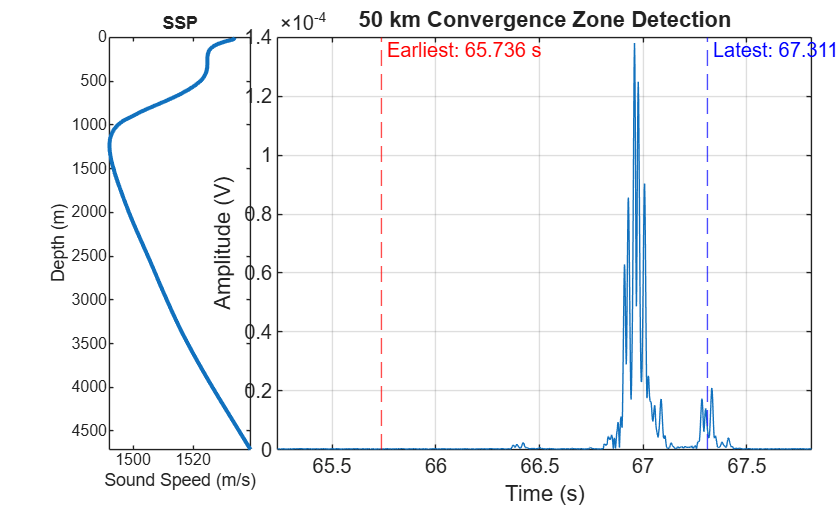
Integrate the pulse-compressed signals non-coherently and plot the result. After matched filtering, the 100 ms chirp is compressed to approximately 10 ms, sharpening each multipath arrival. The echo arrives at approximately 66.9 s with individual forward/return path combinations now appearing as distinct, narrower peaks.

rxInt = pulsint(rxPulses,"noncoherent");

twoWayDelay = min(arrivalsForward.PathDelay) + min(arrivalsReturn.PathDelay);
maxTwoWay = max(arrivalsForward.PathDelay) + max(arrivalsReturn.PathDelay);

plot(t, abs(rxInt))
grid on
xlabel("Time (s)")
ylabel("Amplitude (V)")
title("50 km Convergence Zone Detection")
xlim([twoWayDelay-0.5 maxTwoWay+0.5])
hold on
xline(twoWayDelay, "r--", sprintf("Earliest: %.3f s", twoWayDelay), ...
    LabelOrientation="horizontal")
xline(maxTwoWay, 'b--', sprintf("Latest: %.3f s", maxTwoWay), ...
    LabelOrientation="horizontal")
hold off

Figure Bellhop Eigenrays contains 2 axes objects. Axes object 1 with title SSP, xlabel Sound Speed (m/s), ylabel Depth (m) contains an object of type line. Axes object 2 with title 50 km Convergence Zone Detection, xlabel Time (s), ylabel Amplitude (V) contains 3 objects of type line, constantline.

fprintf("Two-way delay range: %.3f - %.3f s (spread: %.1f ms)\n", ...
    twoWayDelay, maxTwoWay, (maxTwoWay-twoWayDelay)*1000)

Two-way delay range: 65.736 - 67.311 s (spread: 1575.1 ms)

fprintf("Target range: %.0f m\n", twoWayDelay*meanSoundSpeed/2)

Target range: 49795 m

Beamformed Reception

The omnidirectional hydrophone receives signal from all directions equally, including noise from every angle and multipath arrival at different elevation angles that spread the echo in time. A vertical line array (VLA) steered toward the dominant arrival provides two benefits:

Improved SNR: The beamformer sums the signal coherently across $N$ elements, while independent noise adds incoherently. This processing provides up to $10 \log_{10} (N)$ dB of array gain against noise.
Reduced multipath spreading: The narrow beam passes only arrivals near the steered direction and rejects off-angle paths. This directional filtering suppresses multipath arrivals that spread the echo in time.

Set up a 32-element VLA with half-wavelength spacing at 1 kHz, steered to the strongest return-leg arrival. The theoretical maximum array gain is $10 \log_{10} (32) \approx 15$ dB, and the beamwidth of approximately 3.6 degrees is narrow enough to discriminate between the different multipath arrival angles.

lambda = meanSoundSpeed/fc;
nElements = 32;

array = phased.ULA('NumElements',nElements, ...
    'ElementSpacing',lambda/2, ...
    'Element',hydro, ...
    'ArrayAxis','z');

directRetDir = arrivalsReturn.AngleOfArrival(1,:)';

arrayCollector = phased.Collector('Sensor',array, ...
    'OperatingFrequency',fc,'PropagationSpeed',meanSoundSpeed);

beamformer = phased.PhaseShiftBeamformer('SensorArray',array, ...
    'OperatingFrequency',fc, ...
    'PropagationSpeed',meanSoundSpeed, ...
    'Direction',directRetDir);

Rerun the simulation with the VLA at the receiver. Noise is applied per element before beamforming so that each element contributes independent thermal noise. The beamformer then coherently sums the element signals: the in-phase signal adds constructively while uncorrelated noise partially cancels.

release(channeFwd)
release(channelRet)

rx_bf = phased.ReceiverPreamp('Gain',20,'NoiseFigure',10, ...
    'SampleRate',fs,'SeedSource','Property','Seed',2007);

mf_bf = phased.MatchedFilter('Coefficients',getMatchedFilter(wav), ...
    'SpectrumWindow','Hamming');

rxbfpulses = zeros(size(x,1), xmits);

for j = 1:xmits
    tsig = x .* proj(fc, srcAngFwd)';
    tsig = channeFwd(tsig, pathsForward, dopplerForward, alossForward);
    tsig = tsig .* phaseForward;
    tsig = tgt(tsig, tgtAngFwd);
    tsigRet = repmat(sum(tsig,2), 1, numRet);
    tsigRet = channelRet(tsigRet, pathsReturn, dopplerReturn, alossReturn);
    tsigRet = tsigRet .* phaseReturn;
    rsig = arrayCollector(tsigRet, rcvAngRet);
    rsig = rx_bf(rsig);
    rsig = beamformer(rsig);
    rxbfpulses(:,j) = mf_bf(rsig);
end

Omnidirectional vs. Beamformed Comparison

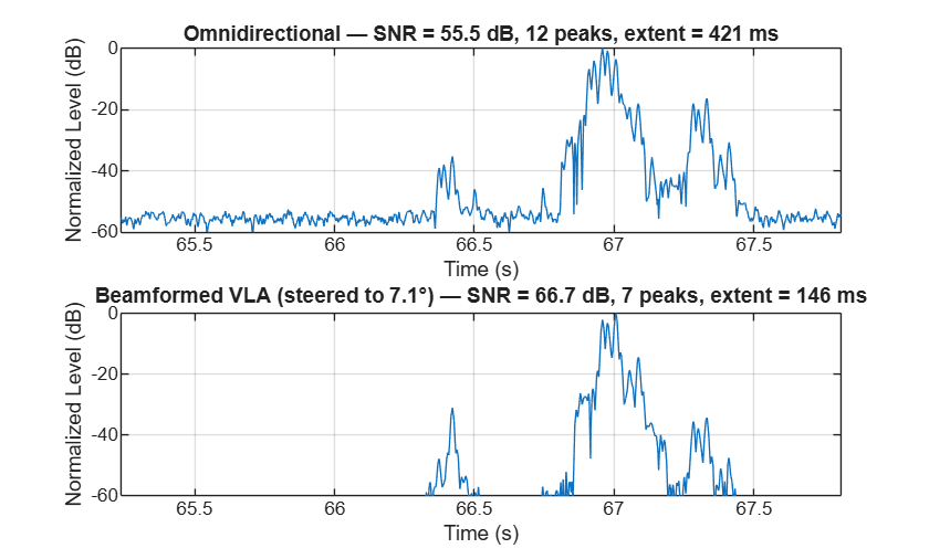
Compare the omnidirectional and beamformed detections. The beamformer provides both SNR improvement and multipath suppression. SNR is measured as peak echo power relative to the noise floor before the echo arrives. Echo extent is measured as the time span containing all peaks above –20 dB relative to the maximum.

rxbfint = pulsint(rxbfpulses,"noncoherent");

echoWindow = t >= twoWayDelay-0.1 & t <= maxTwoWay+0.1;
noiseWindow = t < twoWayDelay-1;

snromni = 10*log10(max(abs(rxInt(echoWindow)).^2) / mean(abs(rxInt(noiseWindow)).^2));
snrbf = 10*log10(max(abs(rxbfint(echoWindow)).^2) / mean(abs(rxbfint(noiseWindow)).^2));

echoRegion = t >= twoWayDelay-0.2 & t <= maxTwoWay+0.2;
tEcho = t(echoRegion);
omniEchoNorm = abs(rxInt(echoRegion)) / max(abs(rxInt(echoRegion)));
bfEchoNorm = abs(rxbfint(echoRegion)) / max(abs(rxbfint(echoRegion)));
[pksOmni, idxOmni] = findpeaks(omniEchoNorm, MinPeakHeight= 10^(-20/20), MinPeakDistance= 20);
[pksbf, idxbf] = findpeaks(bfEchoNorm, MinPeakHeight= 10^(-20/20), MinPeakDistance= 20);
extentOmni = (tEcho(idxOmni(end)) - tEcho(idxOmni(1))) * 1000;
extentbf = (tEcho(idxbf(end)) - tEcho(idxbf(1))) * 1000;

subplot(2,1,1)
plot(t, mag2db(abs(rxInt)/max(abs(rxInt))))
grid on
xlabel("Time (s)")
ylabel("Normalized Level (dB)")
title(sprintf("Omnidirectional — SNR = %.1f dB, %d peaks, extent = %.0f ms", ...
    snromni, length(pksOmni), extentOmni))
xlim([twoWayDelay-0.5 maxTwoWay+0.5])
ylim([-60 0])

subplot(2,1,2)
plot(t, mag2db(abs(rxbfint)/max(abs(rxbfint))))
grid on
xlabel("Time (s)")
ylabel("Normalized Level (dB)")
title(sprintf("Beamformed VLA (steered to %.1f\\circ) — SNR = %.1f dB, %d peaks, extent = %.0f ms", ...
    directRetDir(2), snrbf, length(pksbf), extentbf))
xlim([twoWayDelay-0.5 maxTwoWay+0.5])
ylim([-60 0])

fprintf(['SNR (omnidirectional): %.1f dB\n' ...
    'SNR (beamformed):      %.1f dB\n' ...
    'Array gain:            %.1f dB (theoretical max: %.1f dB)\n' ...
    'Echo extent (omni):    %.0f ms (%d peaks above -20 dB)\n' ...
    'Echo extent (BF):      %.0f ms (%d peaks above -20 dB)\n' ...
    'Spread reduction:      %.0f%%\n'], ...
    snromni, snrbf, snrbf - snromni, 10*log10(nElements), ...
    extentOmni, length(pksOmni), extentbf, length(pksbf), ...
    (1 - extentbf/extentOmni)*100)

SNR (omnidirectional): 55.5 dB
SNR (beamformed):      66.7 dB
Array gain:            11.1 dB (theoretical max: 15.1 dB)
Echo extent (omni):    421 ms (12 peaks above -20 dB)
Echo extent (BF):      146 ms (7 peaks above -20 dB)
Spread reduction:      65%

Summary

This example demonstrated an active sonar simulation using Bellhop over the Bermuda Rise region in the North Atlantic. A sound speed profile computed using WOA 2023 temperature and salinity data captures the essential deep-ocean SOFAR channel structure (axis near 1250 m depth), enabling convergence zone detection at ranges where simple spherical spreading predicts much higher losses. A VLA steered toward the dominant arrival at the receiver improves the received SNR by approximately 11 dB and reduces multipath spreading by 65%.

References

[1] Jensen, F.B., Kuperman, W.A., Porter, M.B., and Schmidt, H. Computational Ocean Acoustics. New York: Springer, 2011.

[2] Reagan, James R.; Boyer, Tim P.; García, Hernán E.; Locarnini, Ricardo A.; Baranova, Olga K.; Bouchard, Courtney; Cross, Scott L.; Mishonov, Alexey V.; Paver, Christopher R.; Seidov, Dan; Wang, Zhankun; Dukhovskoy, Dmitry (2023). World Ocean Atlas 2023. Temperature and Salinity. NOAA National Centers for Environmental Information. Data set. https://doi.org/10.25921/va26-hv25. Accessed June 29th, 2026.

[3] Locarnini, R.A., A.V. Mishonov, O.K. Baranova, J.R. Reagan, T.P. Boyer, D. Seidov, Z. Wang, H.E. Garcia, C. Bouchard, S.L. Cross, C.R. Paver, and D. Dukhovskoy (2024). World Ocean Atlas 2023, Volume 1: Temperature. A. Mishonov Technical Editor, NOAA Atlas NESDIS 89. https://doi.org/10.25923/54bh-1613

[4] Reagan, J.R., D. Seidov, Z. Wang, D. Dukhovskoy, T.P. Boyer, R.A. Locarnini, O.K. Baranova, A.V. Mishonov, H.E. Garcia, C. Bouchard, S.L. Cross, and C.R. Paver. (2024). World Ocean Atlas 2023, Volume 2: Salinity. A. Mishonov, Technical Editor, NOAA Atlas NESDIS 90. https://doi.org/10.25923/70qt-9574

[5] GEBCO Bathymetric Compilation Group 2026, 'The GEBCO_2026 Grid — a continuous terrain model for oceans and land at 15 arc-second intervals,' NERC EDS British Oceanographic Data Centre NOC, 2026. doi:10.5285/4f68d5c7-45eb-f999-e063-7086abc036fa