Introduction to Differential Beamforming
This example shows the basic concept of differential beamforming and how to use that technology to form a linear differential microphone array.
Additive vs. Differential Microphone Arrays
Microphone arrays have been deployed in many audio applications. Depending on the layout, microphone arrays can be divided into two main categories: additive microphone arrays and differential microphone arrays. The additive microphone arrays are similar to the arrays used in other applications, like wireless communications. For an additive microphone array, the goal is to coherently combine the signals from each channel so we can form a narrow beam towards the source and improve the signal to noise ratio. Several such beamforming algorithms are covered in the Acoustic Beamforming Using a Microphone Array example.
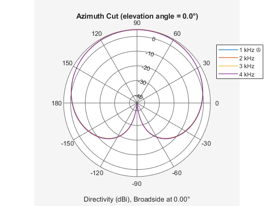
Although additive microphone arrays are very useful, they suffer from several limitations. For illustration purpose, let us define a 2-element array with a 5 cm spacing and look at its pattern between 1-4 kHz. Note that although the audio frequency band spans from 20 Hz to 20 kHz, the 1-4 kHz bands are particularly important for speech intelligibility. The 5 cm spacing in the array is approximately half wavelength at 4 kHz.
c = 343;
f = (1:4)*1e3;
fmax = f(end);
lambda = c/fmax;

d = 0.05;
N = 2;
micarraya = phased.ULA(N,d);

pattern(micarraya,f,-180:180,0,'PropagationSpeed',c)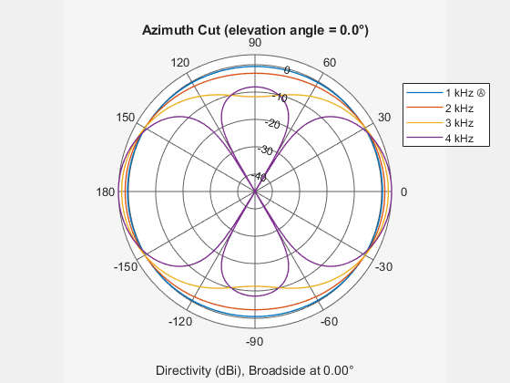
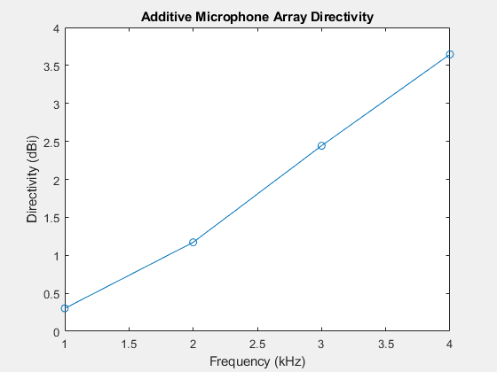
The first thing we can observe from the plots is probably how much the pattern changed across this frequency range. Although the array exhibits a clear directional response at 4 kHz, at 1 kHz, its pattern is essentially omnidirectional. As a result, at lower frequencies, the array cannot achieve much spatial filtering. This, in turn, reduces the directivity of the array. The directivity along the broadside across the frequency range is captured below.
Da = directivity(micarraya,f,[0;0],'PropagationSpeed',c);
clf;
plot(f/1e3,Da,'-o');
xlabel('Frequency (kHz)');
ylabel('Directivity (dBi)');
title('Additive Microphone Array Directivity');
Note that the signal of interest for a microphone array, such as speech and music, is always wideband. Therefore, the pattern difference across the frequency range also causes distortions on the beamformed signal.
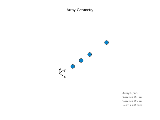
Many array geometries have been explored to get around these limitations. A nested array is one such example. In a nested array, small arrays are embedded in a large array. You can then activate different elements across different frequency bands to produce similar patterns across the band. Consider the following 4-element array
Nn = 4;
nestedpos = [zeros(1,Nn);[0 1 2 4]*d;zeros(1,Nn)];
micarrayn = phased.ConformalArray('ElementPosition',nestedpos);
viewArray(micarrayn);
set(gcf,'Color','w');
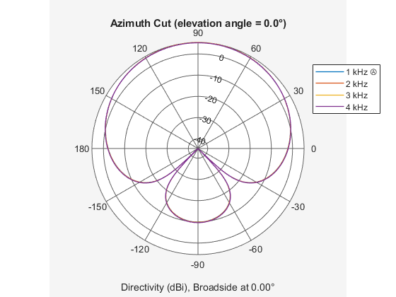
If you use the first and the second elements for bands around 4 kHz; the first and the third elements for bands between 2 and 3 kHz; and the first and the fourth elements for bands around 1 kHz, the resulting beam patterns look like
wn = [1 1 1 1;0 0 0 1;0 1 1 0;1 0 0 0];
pattern(micarrayn,f,-180:180,0,'PropagationSpeed',c,'Weights',wn);
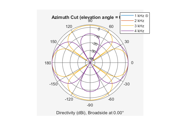
In the plot the patterns from 1, 2, and 4 kHz are essentially identical to each other, but the 3kHz pattern is still different. In addition, the number of elements are doubled in this design. In reality, to get a nested array that can have a frequency invariant pattern across a large band, you will need a large number of microphone elements, so this approach is not very practical.
Differential microphone array (DMA) technology is another possible solution. Because DMAs can form frequency invariant patterns, they become valuable tools for audio applications.
First Order Linear DMA
Unlike an additive microphone array, a DMA is more sensitive to the spatial derivative of the acoustic field around the array, thus the name "differential". Since it is impossible to compute the true derivative between microphone elements, the difference between the measurements at each microphone element is used to approximate the derivative. Because a pair of closely located elements can measure derivative more accurately, the element spacing in a DMA is in general much smaller than the wavelength. The following code constructs a 2-element linear array with a spacing of 1/10 wavelength.
dd = lambda/10;
micarrayd = phased.ULA(N,dd);
viewArray(micarrayd)
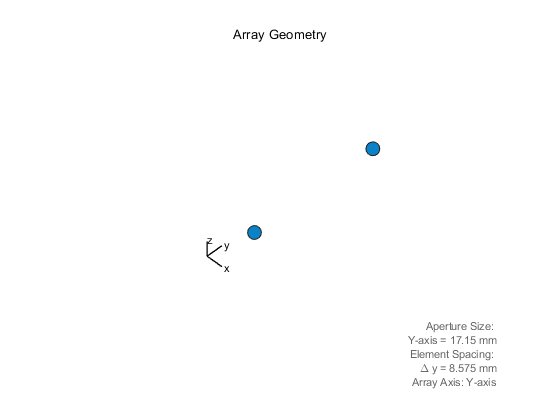
set(gcf,'Color','w');
One benefit comes with a close spacing is that the entire array aperture is fairly small. As a result, such linear DMAs are popular choices for hearing aids.
Because differential beamforming measures the field derivatives, its mainlobe points toward the endfire direction. The endfire direction is along the axis of the linear array. This is understandable because for an additive array, the mainlobe is at the broadside, which is the direction perpendicular to the array axis, and the derivative at that direction is 0. Therefore, the design of a DMA is often about null placement. For a two-element linear DMA, when the mainlobe is at endfire, you can only control one null location. This is referred to as a first order DMA. However, even though there is only one null location, varying the location can result in several interesting patterns.
First, put the null at the broadside of the array. This means that we need to compute a weight vector, when combined with the steering vectors for endfire and broadside directions, to generate unit response and null response, respectively. Such a weight vector can be derived using a least square approach.
ang_d = 90;  % endfire
ang_n = 0;   % broadside
dd_f = dd./(c./f);
w = complex(zeros(N,numel(f)));
for m = 1:numel(f)
    w(:,m) = diffbfweights(N,dd_f(m),ang_n,'ArrayGeometry','ULA');
end

clf;
pattern(micarrayd,f,-180:180,0,'PropagationSpeed',c,'Weights',w);
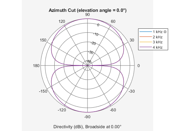
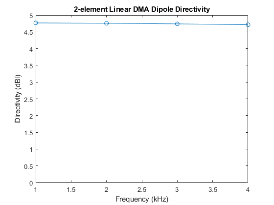
The resulting pattern has the shape of a dipole. Note that the patterns from all frequencies are overlap so they are invariant across the entire frequency band. The directivities are now a constant over the frequency, as shown in the following figure.
Dd = directivity(micarrayd,f,ang_d,'PropagationSpeed',c,'Weights',w);
clf;
plot(f/1e3,Dd,'-o');
ylim([0 5]);
xlabel('Frequency (kHz)');
ylabel('Directivity (dBi)');
title('2-element Linear DMA Dipole Directivity');
Another important performance characteristic associated with a microphone array is its signal to noise ratio (SNR) gain over white noise.
agd = phased.ArrayGain('SensorArray',micarrayd,'PropagationSpeed',c,'WeightsInputPort',true);
wngd = agd(f,ang_d,w);
clf;
plot(f/1e3,wngd,'-*');
xlabel('Frequency (kHz)');
ylabel('White Noise Gain (dB)');
title('2-element Linear DMA Dipole SNR Gain');
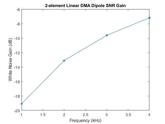
As can be seen from the plot, the SNR gain of this DMA is below 0 dB across the entire frequency range, this means that the noise gets amplified significantly, especially in low frequency regions. Compared to additive arrays, this is probably the biggest issue associated with DMAs. Therefore, engineers may need to make a tradeoff between a more focused beam, which helps dealing with reverberation in a crowded environment, and a higher received signal SNR.
What if the null is located at the other end of the endfire direction?
ang_n = -90;   % endfire
for m = 1:numel(f)
    w(:,m) = diffbfweights(N,dd_f(m),ang_n,'ArrayGeometry','ULA');
end

pattern(micarrayd,f,-180:180,0,'PropagationSpeed',c,'Weights',w);
Now the resulting pattern is a cardioid. You can also put the null at -45 degrees to get a supercardioid shape.
ang_n = -45;   % endfire
for m = 1:numel(f)
    w(:,m) = diffbfweights(N,dd_f(m),ang_n,'ArrayGeometry','ULA');
end

pattern(micarrayd,f,-180:180,0,'PropagationSpeed',c,'Weights',w);
wngd = agd(f,ang_d,w);
clf;
plot(f/1e3,wngd,'-*');
xlabel('Frequency (kHz)');
ylabel('White Noise Gain (dB)');
title('2-element Linear DMA Supercardioid SNR Gain');
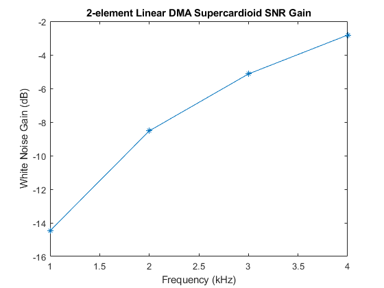
Note that supercardioid shape provides better SNR gain than the dipole shape.
Higher Order Linear DMA
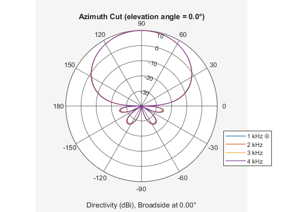
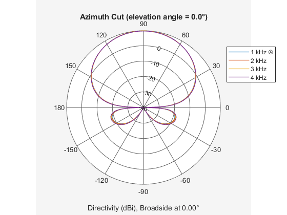
You probably have noticed that for a first order linear DMAs, you can assign 1 null direction. In general, an N-element linear array can form an (N-1)-th order DMA, with the capability of allocating N-1 nulls. For example, for a four-microphone, third order DMA, you can put 3 nulls for the supercardioid beam pattern.
N = 4;
micarrayd3 = phased.ULA(N,dd);
ang_d = 90;            % endfire
ang_n = [0 -30 -90];   % nulls
w = complex(zeros(N,numel(f)));
for m = 1:numel(f)
    w(:,m) = diffbfweights(N,dd_f(m),ang_n,'ArrayGeometry','ULA');
end

pattern(micarrayd3,f,-180:180,0,'PropagationSpeed',c,'Weights',w);
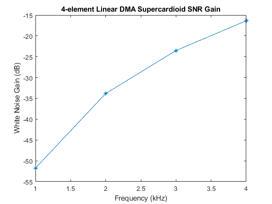
The SNR gain of higher oder DMAs still bears the same trend as a first order DMA.
agd = phased.ArrayGain('SensorArray',micarrayd3,'PropagationSpeed',c,'WeightsInputPort',true);
wngd = agd(f,ang_d,w);
clf;
plot(f/1e3,wngd,'-*');
xlabel('Frequency (kHz)');
ylabel('White Noise Gain (dB)');
title('4-element Linear DMA Supercardioid SNR Gain');
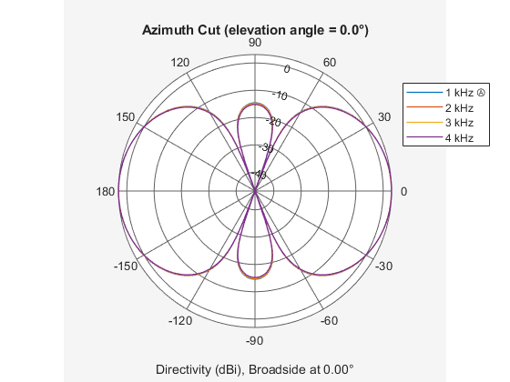
It is possible to assign nulls with multiplicity too. Here is an example where you set the null at -90 degrees to a multiplicity of 2.
ang_n = [0 -90 -90];   % nulls
w = complex(zeros(N,numel(f)));
for m = 1:numel(f)
    w(:,m) = diffbfweights(N,dd_f(m),ang_n,'ArrayGeometry','ULA');
end

pattern(micarrayd3,f,-180:180,0,'PropagationSpeed',c,'Weights',w);
Although the endfire mainlobe of a default DMA works well for hearing aid applications, it is not ideal for other applications such as a sound bar. In those applications, you probably would expect the main beam to be more or less steered toward the broadside of the array. However, although a linear DMA can be steered, it has several unique characteristics compared to an additive array:
The steering sacrifices degree of freedoms from the array. For an L-th order linear DMA, you can at most specify L-1 nulls, the remaining null is picked by algorithm based on the specified null locations. Therefore, a first order linear DMA is not steerable.
Unlike an additive array, the beam shape of a linear DMA is not preserved when steered.
The following snippet shows how to steer a linear DMA. In this case, the main beam is steered towards the broadside. In addition, a null is placed at 70 degrees off the broadside. The remaining null is derived by the steering weights algorithm.
ang_d = 0;    % broadside
ang_n = 70;   % nulls
w = complex(zeros(N,numel(f)));
for m = 1:numel(f)
    w(:,m) = diffbfweights(N,dd_f(m),ang_n,'ArrayGeometry','ULA','SteerAngle',ang_d);
end

pattern(micarrayd3,f,-180:180,0,'PropagationSpeed',c,'Weights',w);
Note that the mainlobe is now toward the broadside direction. Due to the symmetry of the linear array, the resulting pattern also has an equivalent backlobe. In some designs, this can be mitigated by adopting a microphone element with small backlobes.
Summary
This example introduced the basic concept of differential microphone arrays. The example showed how to compute the differential beamforming weights to form many classic DMA beam shapes and compared the performance of a linear DMA with a linear additive microphone array. The array beam pattern clearly illustrated that the DMA can provide a frequency invariant pattern. The example ends with a discussion on how to steer a higher order linear DMA.
References
[1] Jingdong Chen, Jacob Benesty, and Chao Pan, On the design and Implementation of Linear Differential Microphone Arrays, The Journal of the Acoustical Society of America, Vol. 136, No. 6, 2014
[2] Jacob Benesty, Jingdong Chen, and Chao Pan, Fundamentals of Differential Beamforming, Springer, 2016.
[3] Jilu Jin et al., Steering Study of Linear Differential Microphone Arrays, IEEE/ACM Transactions on Audio Speech, and Language Processing, Vol. 29, 2021