Radar and Communications Waveform Classification Using Deep Learning

Generate Radar Waveforms

Generate 3000 signals with a sample rate of 100 MHz for each modulation type. Use phased.RectangularWaveform for rectangular pulses, phased.LinearFMWaveform for LFM, and phased.PhaseCodedWaveform for phase coded pulses with Barker code.

Each signal has unique parameters and is augmented with various impairments to make it more realistic. For each waveform, the pulse width and repetition frequency will be randomly generated. For LFM waveforms, the sweep bandwidth and direction are randomly generated. For Barker waveforms, the chip width and number are generated randomly. All signals are impaired with white Gaussian noise using the awgn function with a random signal-to-noise ratio in the range of [–6, 30] dB. A frequency offset with a random carrier frequency in the range of [Fs/6, Fs/5] is applied to each signal using the comm.PhaseFrequencyOffset object. Lastly, each signal is passed through a multipath Rician fading channel, comm.RicianChannel.

The helper function helperGenerateRadarWaveforms creates and augments each modulation type.

rng default
[wav, modType] = helperGenerateRadarWaveforms();

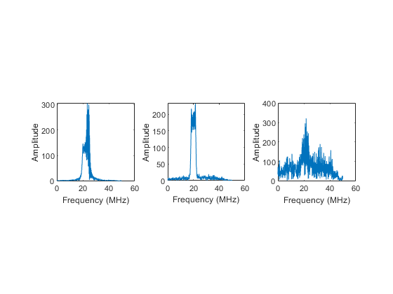
Plot the Fourier transform for a few of the LFM waveforms to show the variances in the generated set.

idLFM = find(modType == "LFM",3);
nfft = 2^nextpow2(length(wav{1}));
f = (0:(nfft/2-1))/nfft*100e6;

figure
subplot(1,3,1)
Z = fft(wav{idLFM(1)},nfft);
plot(f/1e6,abs(Z(1:nfft/2)))
xlabel('Frequency (MHz)');ylabel('Amplitude');axis square
subplot(1,3,2)
Z = fft(wav{idLFM(2)},nfft);
plot(f/1e6,abs(Z(1:nfft/2)))
xlabel('Frequency (MHz)');ylabel('Amplitude');axis square
subplot(1,3,3)
Z = fft(wav{idLFM(3)},nfft);
plot(f/1e6,abs(Z(1:nfft/2)))
xlabel('Frequency (MHz)');ylabel('Amplitude');axis square

Feature Extraction Using Wigner-Ville Distribution

To improve the classification performance of machine learning algorithms, a common approach is to input extracted features in place of the original signal data. The features provide a representation of the input data that makes it easier for a classification algorithm to discriminate across the classes. The Wigner-Ville distribution represents a time-frequency view of the original data that is useful for time varying signals. The high resolution and locality in both time and frequency provide good features for the identification of similar modulation types. Use the wvd function to compute the smoothed pseudo WVD for each of the modulation types.

figure
subplot(1,3,1)
wvd(wav{find(modType == "Rect",1)},100e6,'smoothedPseudo')
axis square; colorbar off; title('Rect')
subplot(1,3,2)
wvd(wav{find(modType == "LFM",1)},100e6,'smoothedPseudo')
axis square; colorbar off; title('LFM')
subplot(1,3,3)
wvd(wav{find(modType == "Barker",1)},100e6,'smoothedPseudo')
axis square; colorbar off; title('Barker')

To store the smoothed-pseudo Wigner-Ville distribution of the signals, first create the directory TFDDatabase inside your temporary directory tempdir. Then create subdirectories in TFDDatabase for each modulation type. For each signal, compute the smoothed-pseudo Wigner-Ville distribution, and downsample the result to a 227-by-227 matrix. Save the matrix as a .png image file in the subdirectory corresponding to the modulation type of the signal. The helper function helperGenerateTFDfiles performs all these steps. This process will take several minutes due to the large database size and the complexity of the wvd algorithm. You can replace tempdir with another directory where you have write permission.

parentDir = tempdir;
dataDir = 'TFDDatabase';
helperGenerateTFDfiles(parentDir,dataDir,wav,modType,100e6)

Create an image datastore object for the created folder to manage the image files used for training the deep learning network. This step avoids having to load all images into memory. Specify the label source to be folder names. This assigns the modulation type of each signal according to the folder name.

folders = fullfile(parentDir,dataDir,{'Rect','LFM','Barker'});
imds = imageDatastore(folders,...
    'FileExtensions','.png','LabelSource','foldernames','ReadFcn',@readTFDForSqueezeNet);

The network is trained with 80% of the data and tested on with 10%. The remaining 10% is used for validation. Use the splitEachLabel function to divide the imageDatastore into training, validation, and testing sets.

[imdsTrain,imdsTest,imdsValidation] = splitEachLabel(imds,0.8,0.1);

Set Up Deep Learning Network

Before the deep learning network can be trained, define the network architecture. This example utilizes transfer learning SqueezeNet, a deep CNN created for image classification. Transfer learning is the process of retraining an existing neural network to classify new targets. This network accepts image input of size 227-by-227-by-3. Prior to input to the network, the custom read function readTFDForSqueezeNet transforms the two-dimensional time-frequency distribution to an RGB image of the correct size. SqueezeNet performs classification of 1000 categories in its default configuration.

Use imagePretrainedNetwork function to load SqueezeNet. Setting the "NumClasses" argument to three will reconfigure the network to classify the input images into three categories.

numClasses = 3;
net = imagePretrainedNetwork("squeezenet","NumClasses",numClasses,"ClassNamesType","string");

Confirm that SqueezeNet is configured for images of size 227-by-227-by-3.

net.Layers(1)

ans = 
  ImageInputLayer with properties:

                      Name: 'data'
                 InputSize: [227 227 3]
        SplitComplexInputs: 0

   Hyperparameters
          DataAugmentation: 'none'
             Normalization: 'zerocenter'
    NormalizationDimension: 'auto'
                      Mean: [1×1×3 single]

Replace the drop9 layer, the last dropout layer in the network, with a dropout layer of probability 0.6.

newDropoutLayer = dropoutLayer(0.6,'Name','new_dropout');
net = replaceLayer(net,'drop9',newDropoutLayer);

Also increase the learning rate factors of the last learnable layer.

net = setLearnRateFactor(net,"conv10/Weights",20);
net = setLearnRateFactor(net,"conv10/Bias",20);

Inspect the last six layers of the network. Confirm that the dropout and the convolutional layer parameters have been changed.

net.Layers(end-5:end)

ans = 
  6×1 Layer array with layers:

     1   'new_dropout'    Dropout                      60% dropout
     2   'conv10'         2-D Convolution              3 1×1×512 convolutions with stride [1  1] and padding [0  0  0  0]
     3   'relu_conv10'    ReLU                         ReLU
     4   'pool10'         2-D Global Average Pooling   2-D global average pooling
     5   'prob'           Softmax                      softmax
     6   'prob_flatten'   Flatten                      Flatten

Choose options for the training process that ensures good network performance. Refer to the trainingOptions documentation for a description of each option.

options = trainingOptions('sgdm', ...
    'MiniBatchSize',128, ...
    'MaxEpochs',5, ...
    'InitialLearnRate',1e-3, ...
    'Shuffle','every-epoch', ...
    'Verbose',false, ...
    'Plots','training-progress',...
    'ValidationData',imdsValidation,...
    'Metrics','accuracy');

Train the Network

Use the trainnet command to train the created CNN. Because the data set is large in size, the process can take several minutes. If your machine has a GPU and Parallel Computing Toolbox™, then MATLAB® automatically uses the GPU for training. Otherwise, it uses the CPU. The training accuracy plots in the figure show the progress of the network's learning across all iterations. On the three radar modulation types, the network classifies almost 100% of the training signals correctly.

trainedNet = trainnet(imdsTrain,net,'crossentropy',options);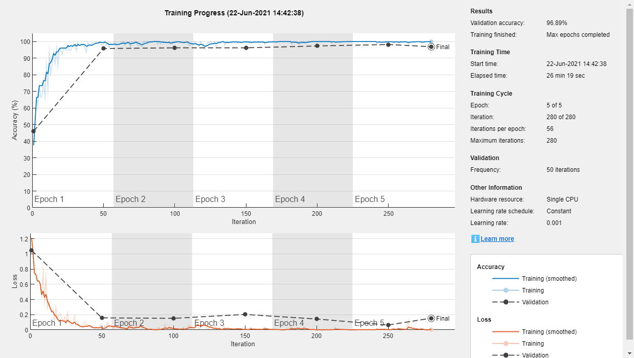

Evaluate Performance on Radar Waveforms

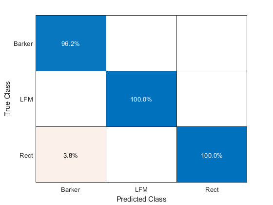
Use the trained network to compute class scores for the testing data using the minibatchpredict command. Then use the scores2label command to convert the computed scores into the class labels. A confusion matrix is one method to visualize classification performance. Use the confusionchart command to calculate and visualize the classification accuracy. For the three modulation types input to the network, almost all of the phase coded, LFM, and rectangular waveforms are correctly identified by the network.

scores = minibatchpredict(trainedNet,imdsTest);
predicted = scores2label(scores,categories(imdsTest.Labels));

figure
confusionchart(imdsTest.Labels,predicted,'Normalization','column-normalized')

Generate Communications Waveforms and Extract Features

The frequency spectrum of a radar classification system must compete with other transmitted sources. See how the created network extends to incorporate other simulated modulation types. Another MathWorks® example, Modulation Classification with Deep Learning (Communications Toolbox), performs modulation classification of several different modulation types using Communications Toolbox™. The helper function helperGenerateCommsWaveforms generates and augments a subset of the modulation types used in that example. Since the WVD loses phase information, a subset of only the amplitude and frequency modulation types is used.

See the example link for an in-depth description of the workflow necessary for digital and analog modulation classification and the techniques used to create these waveforms. For each modulation type, use wvd to extract time-frequency features and visualize.

[wav, modType] = helperGenerateCommsWaveforms();

figure
subplot(2,3,1)
wvd(wav{find(modType == "GFSK",1)},200e3,'smoothedPseudo')
axis square; colorbar off; title('GFSK')
subplot(2,3,2)
wvd(wav{find(modType == "CPFSK",1)},200e3,'smoothedPseudo')
axis square; colorbar off; title('CPFSK')
subplot(2,3,3)
wvd(wav{find(modType == "B-FM",1)},200e3,'smoothedPseudo')
axis square; colorbar off; title('B-FM')
subplot(2,3,4)
wvd(wav{find(modType == "SSB-AM",1)},200e3,'smoothedPseudo')
axis square; colorbar off; title('SSB-AM')
subplot(2,3,5)
wvd(wav{find(modType == "DSB-AM",1)},200e3,'smoothedPseudo')
axis square; colorbar off; title('DSB-AM')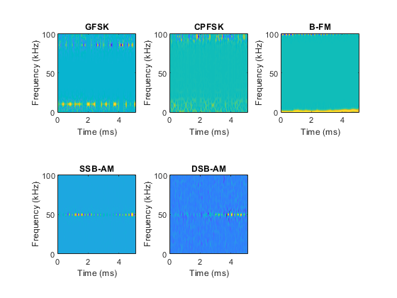

Use the helper function helperGenerateTFDfiles again to compute the smoothed pseudo WVD for each input signal. Create an image datastore object to manage the image files of all modulation types.

helperGenerateTFDfiles(parentDir,dataDir,wav,modType,200e3)
folders = fullfile(parentDir,dataDir,{'Rect','LFM','Barker','GFSK','CPFSK','B-FM','SSB-AM','DSB-AM'});
imds = imageDatastore(folders,...
    'FileExtensions','.png','LabelSource','foldernames','ReadFcn',@readTFDForSqueezeNet);

Again, divide the data into a training set, a validation set, and a testing set using the splitEachLabel function.

rng default
[imdsTrain,imdsTest,imdsValidation] = splitEachLabel(imds,0.8,0.1);

Adjust Deep Learning Network Architecture

Previously, the network architecture was set up to classify three modulation types. This must be updated to allow classification of all eight modulation types of both radar and communication signals. This is a similar process as before, with the exception that the total number of classes is now eight.

numClasses = 8;
net = imagePretrainedNetwork("squeezenet","NumClasses",numClasses,"ClassNamesType","string");

newDropoutLayer = dropoutLayer(0.6,'Name','new_dropout');
net = replaceLayer(net,'drop9',newDropoutLayer);

net = setLearnRateFactor(net,"conv10/Weights",20);
net = setLearnRateFactor(net,"conv10/Bias",20);

Create a new set of training options.

options = trainingOptions('sgdm', ...
    'MiniBatchSize',150, ...
    'MaxEpochs',10, ...
    'InitialLearnRate',1e-4, ...
    'Shuffle','every-epoch', ...
    'Verbose',false, ...
    'Plots','training-progress',...
    'ValidationData',imdsValidation,...
    'Metrics','accuracy');

Use the trainnet command to train the created CNN. For all modulation types, the training converges with an accuracy of about 95% correct classification.

trainedNet = trainnet(imdsTrain,net,'crossentropy',options);

Evaluate Performance on All Signals

Use the minibatchpredict and scores2label commands to classify the signals held aside for testing. Again, visualize the performance using confusionchart.

scores = minibatchpredict(trainedNet,imdsTest);
predicted = scores2label(scores,categories(imdsTest.Labels));

figure;
confusionchart(imdsTest.Labels,predicted,'Normalization','column-normalized')

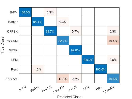
For the eight modulation types input to the network, about 98% of B-FM, CPFSK, GFSK, Barker, and LFM modulation types were correctly classified. On average, about 85% of AM signals were correctly identified. From the confusion matrix, a high percentage of SSB-AM signals were misclassified as DSB-AM and DSB-AM signals as SSB-AM.

Investigate a few of these misclassifications to gain insight into the network's learning process. Use the readimage function on the image datastore to extract from the test dataset a single image from each class. The displayed WVD visually looks very similar. Since DSB-AM and SSB-AM signals have a very similar signature, this explains in part the network's difficulty in correctly classifying these two types. Further signal processing could make the differences between these two modulation types clearer to the network and result in improved classification.

DSB_DSB = readimage(imdsTest,find((imdsTest.Labels == 'DSB-AM') & (predicted == 'DSB-AM'),1));
DSB_SSB = readimage(imdsTest,find((imdsTest.Labels == 'DSB-AM') & (predicted == 'SSB-AM'),1));
SSB_DSB = readimage(imdsTest,find((imdsTest.Labels == 'SSB-AM') & (predicted == 'DSB-AM'),1));
SSB_SSB = readimage(imdsTest,find((imdsTest.Labels == 'SSB-AM') & (predicted == 'SSB-AM'),1));

figure
subplot(2,2,1)
imagesc(DSB_DSB(:,:,1))
axis square; title({'Actual Class: DSB-AM','Predicted Class: DSB-AM'})
subplot(2,2,2)
imagesc(DSB_SSB(:,:,1))
axis square; title({'Actual Class: DSB-AM','Predicted Class: SSB-AM'})
subplot(2,2,3)
imagesc(SSB_DSB(:,:,1))
axis square; title({'Actual Class: SSB-AM','Predicted Class: DSB-AM'})
subplot(2,2,4)
imagesc(SSB_SSB(:,:,1))
axis square; title({'Actual Class: SSB-AM','Predicted Class: SSB-AM'})

Summary

This example showed how radar and communications modulation types can be classified by using time-frequency techniques and a deep learning network. Further efforts for additional improvement could be investigated by utilizing time-frequency analysis available in Wavelet Toolbox™ and additional Fourier analysis available in Signal Processing Toolbox™.

References

[1] Brynolfsson, Johan, and Maria Sandsten. "Classification of one-dimensional non-stationary signals using the Wigner-Ville distribution in convolutional neural networks." 25th European Signal Processing Conference (EUSIPCO). IEEE, 2017.

[2] Liu, Xiaoyu, Diyu Yang, and Aly El Gamal. "Deep neural network architectures for modulation classification." 51st Asilomar Conference on Signals, Systems and Computers. 2017.

[3] `Wang, Chao, Jian Wang, and Xudong Zhang. "Automatic radar waveform recognition based on time-frequency analysis and convolutional neural network." IEEE International Conference on Acoustics, Speech and Signal Processing (ICASSP). 2017.