LPI Radar Waveform Classification Using Time-Frequency CNN

Introduction

LPI radar systems are designed to evade detection by employing specific modulation schemes and transmitting across wide frequency bands at low power levels. In modern LPI radars these conditions are typically achieved by transmitting a continuous-wave (CW) waveform. Detection and classification of LPI waveforms represents a significant challenge. Recent advancements show that deep learning methods can be successfully applied to radar waveform classification. The Radar and Communications Waveform Classification Using Deep Learning (Radar Toolbox) example shows how to classify some standard radar and communications waveforms using a deep CNN. Similar techniques have also been effectively applied to LPI waveforms [1, 2].

This example shows how to classify LPI radar waveforms using a time-frequency CNN. The network accepts a baseband-sampled received radar waveform as input, and outputs the identified class of the waveform (waveform's modulation scheme). The time-frequency CNN used in this example has hidden layers that automatically transform the input time domain signals into time-frequency images by computing the Short Time Fourier Transform (STFT) and the Continuous Wavelet Transform (CWT). This eliminates the need for initial prepossessing or feature extraction.

The example starts by generating a synthetic data set with nine distinct waveform classes customized to simulate transmissions by an LPI radar. These include both linear and non-linear FM waveforms, chirplike phase-coded waveforms, phase-coded waveform based on pseudorandom sequences, as well as an Orthogonal Frequency Division Multiplexing (OFDM) waveform. All waveforms are CW (unit duty cycle) and have wide bandwidths and substantial time-bandwidth products. The training data set also simulates variations in frequency offset and SNR to emulate conditions of a non-cooperative intercept receiver. Additionally, the dataset includes a class of noise-only signals for comprehensive training.

Following data set preparation, the example shows the training process and evaluates classification performance of the trained network for different SNR values.

Time-Frequency Features

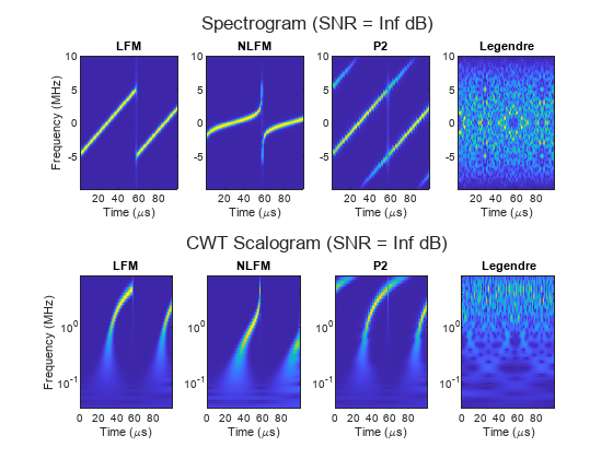
Conventional radar pulse compression techniques employ FM or PM to produce pulses that exhibit a high time-bandwidth product, which is essential for achieving high range resolution. The particular modulation technique applied to a pulse shapes its distinct time-frequency profile. Consequently, the modulation scheme of a waveform can be discerned through its unique time-frequency signature. Difference in the time-frequency behavior of waveforms with different modulation schemes is evident when observing the corresponding spectrograms and CWT scalograms. This is the main motivation for using STFT and CWT features to classify radar waveforms.

tau = 0.1e-3;                % Signal duration (s)
B = 10e6;                    % Pulse bandwidth (Hz)
TB = [576 576 576 571];      % Time-bandwidth product for waveforms in waveformTypes
Fs = 20e6;                   % Sample rate (Hz)

helperTimeFrequencyComparison(["LFM", "NLFM", "P2", "Legendre"], tau, B, TB, Fs);

Training Data Set

This example uses synthetic data to train a time-frequency convolutional network for LPI radar waveform classification. The generated training data set contains the following waveforms:

waveformClasses = ["LFM", "NLFM", "Frank", "P1", "P2", "P3", "P4", "MLS", "Legendre", "OFDM"];

Waveform Parameters

The LPI waveform classification occurs at a non-cooperative intercept receiver located at some unknown distance away from the radar. Therefore, the synthesized data must be representative of conditions at an intercept receiver. Assume that the intercept receive bandwidth is 20 MHz and that the network classifies 204.8 $\mu$s long sections of a radar signal. The sample rate is set to be equal to the receive bandwidth, thus each 204.8 $\mu$s long signal is represented by a 4096-element vector.

interceptBandwidth = 20e6;
waveformDuration = 204.8e-6;

The example assumes that the intercept receiver does not know the exact carrier frequency, bandwidth, pulse width, and SNR of a received waveform. These uncertainties are included into the training data set by randomly varying the corresponding parameters.

Uncertainty in the knowledge of the carrier frequency is modeled by a random frequency offset applied to each received waveform. The maximum frequency offset is set to 1 MHz.

maxFrequencyOffset = 1e6;

To make the training data set representative of waveforms with different bandwidths, for each waveform realization the waveform bandwidth is picked uniformly at random from a set of bandwidth values.

waveformBandwidth = [5e6 8e6 10e6 12e6 15e6];

Similarly, the pulse repetition period is varied by varying the time-bandwidth product. Sets of time-bandwidth product values are selected for each waveform class such that they are similar across all considered waveform classes. The possible values are organized in a dictionary object for convenience.

% For the phase-coded waveforms the time-bandwidth product is determined by
% the code sequence length. For Frank, P1, and P2 the sequence length
% must be a perfect square.
timeBandwidthProduct = dictionary(["Frank", "P1", "P2", "P3", "P4"], ...
    repmat({[576 784 1024]}, 1, 5));

% Use the same values for LFM, NLFM, and OFDM.
timeBandwidthProduct = timeBandwidthProduct.insert("LFM", {[576 784 1024]});
timeBandwidthProduct = timeBandwidthProduct.insert("NLFM", {[576 784 1024]});
timeBandwidthProduct = timeBandwidthProduct.insert("OFDM", {[576 784 1024]});

% For MLS the time-bandwidth product values (sequence lengths) are limited
% to 2^n-1.
timeBandwidthProduct = timeBandwidthProduct.insert("MLS", {[511 1023]});

% For Legendre sequences the time-bandwidth product (sequence length) must
% be a prime.
timeBandwidthProduct = timeBandwidthProduct.insert("Legendre", {[571 773 1021]});

The SNR of the intercepted waveform must also vary across the training data set to model variations in the radar (peak power, antenna gain, etc.) and the propagation (distance, atmospheric loss, etc.) parameters. For each training signal realization, the SNR is picked uniformly at random from a set of SNR values.

SNR = -9:3:12;

The training data set also includes noise only samples as a separate class. This is needed to verify the detection capability of the resulting classifier, that is an ability to discriminate between signals that contain a radar waveform and signals that contain noise only.

waveformClasses = [waveformClasses "Noise Only"];
timeBandwidthProduct = timeBandwidthProduct.insert("Noise Only", {[]});

The parameter values selected for the data set generation are summarized in the table below.

Data Generation

Generate a training data set such that each class is represented by 16000 signal realizations.

numTrainSignalsPerClass = 16e3;
saveFolder = tempdir;
trainSetDirectory = fullfile(saveFolder, "SyntheticLPIRadarWaveforms");

% Regenerate the training data set or download it from a repository.
% Note, generating the waveform data set can take a considerable amount of
% time.
useDownloadedDataSet = true;

if ~useDownloadedDataSet
    mkdir(trainSetDirectory);
    for indWaveform = 1:numel(waveformClasses)
        waveformName = waveformClasses(indWaveform);
    
        fprintf("Generating %s samples.\n", waveformName);

        % Generate train signals for waveformName class
        trainData = helperGenerateWaveform(numTrainSignalsPerClass, waveformName, waveformDuration,...
            waveformBandwidth, timeBandwidthProduct{waveformName}, maxFrequencyOffset, interceptBandwidth, SNR);
    
        % Save each signal in a separate .mat file
        helperSaveWaveforms(trainData, trainSetDirectory, waveformName);
    end
else
    % Download file size is 10.3 GB
    dataURL = 'https://ssd.mathworks.com/supportfiles/phased/data/SyntheticLPIRadarWaveforms.zip';
    zipFile = fullfile(saveFolder, 'SyntheticLPIRadarWaveforms.zip');

    if ~exist(zipFile, 'file')
        % Download
        websave(zipFile, dataURL);
    end

    % Unzip the data
    unzip(zipFile, saveFolder);
end

LPI Radar and Interception Range

To put the selected waveform parameters into context, consider an LPI radar system operating at wavelength $$\lambda$$ and a peak transmit power of $$P_t$$. Also consider an intercept receiver with a bandwidth $$B_i$$ located at a distance of $$R_i$$ from the radar. Let the radar transmit and receive antenna gains be equal to $$G_{txrx}$$. Given the SNR at the intercept receiver is equal to some value $$SN{R}_i$$, the distance $$R_i$$ is

where $$\underset{}{\overset{\sim }{G_{txrx}}}$$ is the radar antenna gain in the direction of the interceptor, $$T_{si}$$ is the system temperature of the intercept receiver, and $$L_i$$ is the cumulative loss term. Note that the range is proportional to the transmit peak power. If the SNR required to detect and classify an intercepted waveform is equal to $$SN{R}_i$$ and the corresponding distance between the radar and the intercept receiver is $$R_i>R_{max}$$, where $$R_{max}$$ is the radar maximum detection range, such radar can be considered a "quiet" radar. For this reason, LPI radars transmit with a low peak power. The range $$R_i$$ is also inversely proportional to the interceptor bandwidth. This bandwidth must match or be greater than the radar bandwidth since its exact value is not available at a non-cooperative interceptor. Therefore, it is also beneficial for the LPI radar to transmit over a wide frequency range. A good practical way of achieving a wide bandwidth with a low peak power is to transmit a CW waveform.

Assume the radar system is operating at 10 GHz, the peak transmit power is 1 W, and the antenna gain is 35 dB. Also assume the signal is transmitted towards the intercept receiver through a -30 dB sidelobe and the intercept receiver has an isotropic antenna. Compute the range $$R_i$$ for the SNR values used in the training waveform data set. Set the losses and the system noise temperature at the intercept receiver to 0 dB and 290 K respectively.

Pt = 1;                        % Radar peak transmit power (W)
lambda = freq2wavelen(10e9);   % Radar operating wavelength
Gtxrx = 35;                    % Radar antenna gain (dB)
SL = -30;                      % Radar antenna sidelobe level (dB)
Gi = 0;                        % Intercept receiver antenna gain (dB)
Tsi = 290;                     % System noise temperature at the intercept receiver (K)
k = physconst("Boltzmann");

% Set the bandwidth of the intercept receiver to the value selected for the
% data set generation
Bi = interceptBandwidth;         

Ri = sqrt((Pt*db2pow(Gtxrx+SL)*db2pow(Gi)*lambda^2)./((4*pi)^2*db2pow(SNR)*k*Tsi*Bi));

In turn, the radar maximum detection range $$R_{max}$$ can be computed using the radar range equation

where $$\tau$$ is the duration of the coherent processing interval (CPI), $$G_{tx}=G_{rx}=G_{txrx}$$ are the transmit and receive antenna gains, $$D_x$$ is the SNR required to make a detection, $$T_{sr}$$ is the system noise temperature of the radar receiver, $$\sigma$$ is the radar cross section (RCS) of a target of interest, and $$L_r$$ is the cumulative loss term. Let the LPI radar bandwidth be within the bandwidth of the intercept receiver and let the coherent processing interval (CPI) be equal to 204.8e-6 s (the waveform duration value used for the data set generation). Compute the maximum detection range of the radar assuming the target RCS is 10 dBsm, the system noise temperature is 290 K, and the cumulative losses are 0 dB.

% Required SNR assuming Pd = 0.9, Pfa = 1e-6, and a Swerling 1
% target
Dx = shnidman(0.9, 1e-6, 1, 1);

Tsr = 290;                     % System noise temperature at the radar receiver (K)
rcs = 10;                      % Target RCS (dBsm)

Rmax = ((Pt*waveformDuration*db2pow(2*Gtxrx + rcs)*lambda^2)./((4*pi)^3*db2pow(Dx)*k*Tsr))^(1/4);

Compare the radar maximum detection range with the range of the intercept receiver.

figure;
hold on;
plot(Ri*1e-3, SNR, 'LineWidth', 2, 'DisplayName', 'SNR at interceptor');
xlabel('Interceptor Range (km)');
ylabel('Interceptor SNR (dB)');

xline(Rmax*1e-3, 'r--', 'LineWidth', 2, 'DisplayName', 'Radar max range');
grid on;
legend;

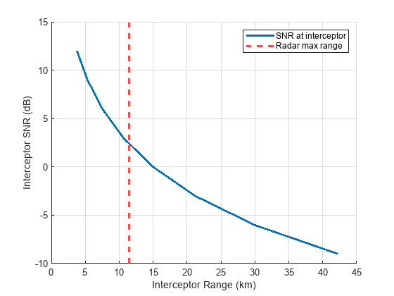
This result shows that the maximum detection range is close to 11.5 km. The SNR at the intercept receiver at this range is 2.5 dB. If the intercept receiver can detect and classify an intercepted radar waveform at this or lower SNR values, the radar can be intercepted at ranges that are beyond its maximum range. If that is the case, the radar is not an LPI radar.

Network Architecture and Training

In this example, a time-frequency CNN is employed to classify received LPI radar signals. The network ingests an input vector consisting of 4096 waveform samples. The first two hidden layers of the network are one-dimensional convolutional layers. They function as adaptable Finite Impulse Response (FIR) filters with learnable impulse responses. The complex input signal is processed by treating the real and imaginary parts as distinct channels.

Tthe architecture of the network splits into two parallel branches. The first branch uses stftLayer to convert the input signal from the time domain into a time-frequency representation by computing spectrograms. Concurrently, the second branch performs a similar transformation, producing a CWT scalogram using cwtLayer (Wavelet Toolbox).

Following the time-frequency transformation, both branches incorporate a sequence of layers commonly found in CNNs designed for image classification. These layers consist of three sets of two-dimensional convolutions, each paired with a Rectified Linear Unit (ReLU) activation function, max pooling, and batch normalization operations.

Upon processing through these stages, the two branches converge, leading to a concatenation of their outputs. This combined feature set then feeds into a series of two densely connected layers, which ultimately culminate in the classification output.

Create the initial layers that consist of an input layer and one-dimensional convolution layers.

numSamples = waveformDuration*interceptBandwidth;

initialLayers = [
    sequenceInputLayer(1, "MinLength", numSamples, "Name", "input", "Normalization", "zscore", "SplitComplexInputs", true)
    convolution1dLayer(7, 2, "stride", 1)
    ];

Create layers for the STFT branch.

stftBranchLayers = [ 
    stftLayer("TransformMode", "squaremag", "Window", hann(64), "OverlapLength", 52, "Name", "stft", "FFTLength", 256, "WeightLearnRateFactor", 0 )
    functionLayer(@(x)dlarray(x, 'SCBS'), Formattable=true, Acceleratable=true, Name="stft_reformat")

    convolution2dLayer([4, 8], 16, "Padding", "same", "Name", "stft_conv_1")
    layerNormalizationLayer("Name", "stft_layernorm_1")
    reluLayer("Name", "stft_relu_1")
    maxPooling2dLayer([4, 8], "Stride", [1 2], "Name", "stft_maxpool_1")  
    
    convolution2dLayer([4, 8], 24, "Padding", "same", "Name", "stft_conv_2")
    layerNormalizationLayer("Name", "stft_layernorm_2")
    reluLayer("Name", "stft_relu_2")
    maxPooling2dLayer([4, 8], "Stride", [1 2], "Name", "stft_maxpool_2")   

    convolution2dLayer([4, 8], 32, "Padding", "same", "Name", "stft_conv_3")
    layerNormalizationLayer("Name", "stft_layernorm_3")
    reluLayer("Name", "stft_relu_3")
    maxPooling2dLayer([4, 8], "Stride", [1 2], "Name", "stft_maxpool_3")

    flattenLayer("Name", "stft_flatten")
    ];

Create layers for the CWT branch.

cwtBranchLayers = [ 
    cwtLayer("SignalLength", numSamples, "TransformMode", "squaremag", "Name","cwt", "WeightLearnRateFactor", 0);
    functionLayer(@(x)dlarray(x, 'SCBS'), Formattable=true, Acceleratable=true, Name="cwt_reformat")

    convolution2dLayer([4, 8], 16, "Padding", "same", "Name", "cwt_conv_1")
    layerNormalizationLayer("Name", "cwt_layernorm_1")
    reluLayer("Name", "cwt_relu_1")
    maxPooling2dLayer([4, 8], "Stride", [1 4], "Name", "cwt_maxpool_1")  
    
    convolution2dLayer([4, 8], 24, "Padding", "same", "Name", "cwt_conv_2")
    layerNormalizationLayer("Name", "cwt_layernorm_2")  
    reluLayer("Name", "cwt_relu_2")
    maxPooling2dLayer([4, 8], "Stride", [1 4], "Name", "cwt_maxpool_2")   

    convolution2dLayer([4, 8], 32, "Padding", "same", "Name", "cwt_conv_3")
    layerNormalizationLayer("Name", "cwt_layernorm_3")    
    reluLayer("Name", "cwt_relu_3")
    maxPooling2dLayer([4, 8], "Stride", [1 4], "Name", "cwt_maxpool_3")   

    flattenLayer("Name", "cwt_flatten")
    ];

Create a set of final fully connected layers.

finalLayers = [
    concatenationLayer(1, 2)
    dropoutLayer(0.5)
    fullyConnectedLayer(48)
    
    dropoutLayer(0.4)
    fullyConnectedLayer(numel(waveformClasses))
    softmaxLayer
    ];

dlLayers = dlnetwork(initialLayers);
dlLayers = addLayers(dlLayers, stftBranchLayers);
dlLayers = addLayers(dlLayers, cwtBranchLayers);
dlLayers = addLayers(dlLayers, finalLayers);

dlLayers = connectLayers(dlLayers, "conv1d", "stft");
dlLayers = connectLayers(dlLayers, "conv1d", "cwt");

dlLayers = connectLayers(dlLayers, "stft_flatten", "concat/in1");
dlLayers = connectLayers(dlLayers, "cwt_flatten", "concat/in2");

Visualize the resulting network.

analyzeNetwork(dlLayers);

Train Time-Frequency CNN

To train the network set trainNow to true, otherwise the example will load a pre-trained network.

trainNow = false;
if trainNow
    % Since the size of the training data set is very large, it cannot all
    % fit into the memory. Set up a signalDatastore object that can
    % efficiently load only that portion of the data set that is required
    % for training at a current iteration.
    waveformDatastore = signalDatastore(trainSetDirectory, "IncludeSubfolders", true);
    
    % Data for each waveform class is stored in a separate directory. The
    % class labels for each waveform realization can conveniently be
    % generated using the directory names.
    labels = folders2labels(waveformDatastore);
    labels = reordercats(labels, waveformClasses);
    labelDatastore = arrayDatastore(labels);
    
    % Create a datastore object that combines both signals and corresponding labels.
    combinedDatastore = combine(waveformDatastore, labelDatastore);
    
    % Set 10 percent of the train data set aside for validation.
    idxs = splitlabels(labels, 0.9);
    trainDatastore = subset(combinedDatastore, idxs{1});
    validationDatastore = subset(combinedDatastore, idxs{2});    
    
    % Specify the training options.
    options = trainingOptions("sgdm", ...
        "InitialLearnRate", 0.001,...
        "MaxEpochs",25, ...
        "MiniBatchSize",100, ...
        "Shuffle","every-epoch",...
        "Plots","training-progress",...
        "ValidationFrequency", 300,...
        "L2Regularization",1e-2,...
        "ValidationData", validationDatastore,...
        "OutputNetwork","best-validation-loss", ...
        "Metric","Accuracy");

    % Train the network. Note, this will take a considerable amount of
    % time.
    net = trainnet(trainDatastore, dlLayers, "crossentropy", options);

else
    % Download file size is 53 MB
    dataURL = 'https://ssd.mathworks.com/supportfiles/phased/data/TimeFrequencyCNNForLPIRadarWaveformClassification.zip';
    zipFile = fullfile(saveFolder, 'TimeFrequencyCNNForLPIRadarWaveformClassification.zip');

    if ~exist(zipFile, 'file')
        % Download
        websave(zipFile, dataURL);
    end  

    % Unzip
    unzip(zipFile, saveFolder);

    % Load the pretrained network
    load(fullfile(saveFolder, 'timeFrequencyCNNForLPIRadarWaveformClassification.mat'));
end

Performance Evaluation

The training dataset includes signals with a range of SNR values to model realistic conditions at a non-cooperative intercept receiver. This also ensures the robustness of the resulting classifier. When assessing the performance of the trained network, it becomes particularly insightful to observe how classification outcomes vary with SNR levels. Good performance of the classifier at low SNR values indicates that a distant intercept receiver can successfully classify an intercepted LPI radar waveform.

To facilitate this analysis, the example creates distinct test datasets for each SNR value. Each of these test datasets comprises 200 test signals per waveform class.

% Number of test signals per waveform class
numTestSignalsPerClassPerSNR = 200;

% Total number of test signals
numTestSignals = numTestSignalsPerClassPerSNR * numel(waveformClasses);
numSNR = numel(SNR);

% True labels for test signals
trueLabels = repmat(waveformClasses, numTestSignalsPerClassPerSNR, 1);
trueLabels = reshape(trueLabels, [], 1);
trueLabels = categorical(trueLabels, waveformClasses);

% Preallocate predicted labels for test signals
predictedLabels = repmat(trueLabels, 1, numSNR);

% Average classification accuracy
averageAccuracy = zeros(numSNR, 1);

% Generate test data for all waveforms but one SNR value at a time
testData = zeros(numSamples, numTestSignals);   
for indSNR = 1:numel(SNR)
    for indWaveform = 1:numel(waveformClasses)
        idxs = (indWaveform-1)*numTestSignalsPerClassPerSNR + 1: indWaveform*numTestSignalsPerClassPerSNR;

        waveformName = waveformClasses(indWaveform); 
        
        testData(:, idxs) = helperGenerateWaveform(numTestSignalsPerClassPerSNR, waveformName, waveformDuration,...
            waveformBandwidth, timeBandwidthProduct{waveformName}, maxFrequencyOffset, interceptBandwidth, SNR(indSNR));
    end

    % Classify test data for SNR(indSNR)
    scores = minibatchpredict(net, num2cell(testData, 1));
    predictedLabels(:, indSNR) = scores2label(scores, waveformClasses);

    % Compute average classification accuracy
    averageAccuracy(indSNR) = nnz(trueLabels == predictedLabels(:, indSNR))/numTestSignals;
end

Plot the average classification accuracy across all classes.

figure;
plot(SNR, averageAccuracy, '--o', 'LineWidth', 2);
xlabel('SNR (dB)');
ylabel('Average Accuracy (%)');
grid on;
title('Average Waveform Classification Accuracy vs. SNR');

The classification performance at low SNR values is poor and reaches only about 45% at -9 dB. However, it starts to improve rapidly after the SNR gets above -3 dB. At SNR of 2.5 dB the average accuracy is close to 83%. This means that in the context of the LPI radar with the maximum range of 11.5 km considered above, the intercept receiver with 2.5 dB SNR at that distance will be able to classify radar waveform with 83% accuracy.

To get more insight into the classification results, plot confusion matrices for different values of SNR.

Plot confusion matrix for SNR = -9 dB.

figure;
confusionchart(trueLabels, predictedLabels(:, 1), 'Normalization', 'row-normalized');
title(sprintf("SNR=%.2f dB", SNR(1)));

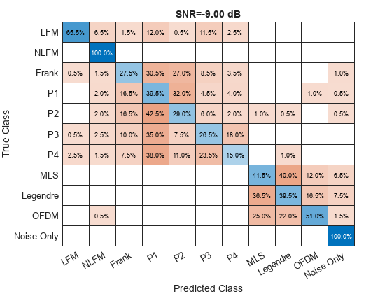
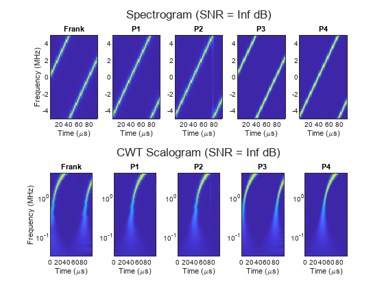
The classifier is having difficulty discriminating between the phase-coded chirplike waveforms, that is Frank, P1, P2, P3, and P4. All these codes approximate phase history of an LFM. Specifically, the Frank code is derived from the phase history of a linearly stepped FM waveform, while P1 and P2 codes are special versions of the Frank code with the DC frequency in the middle of the pulse instead of the beginning [3]. For this reason, these waveforms have almost identical time-frequency behavior, resulting in a high degree of confusion between the corresponding classes. To observe how similar are the time-frequency features of phase-coded chirplike waveforms, plot their spectrograms, scalograms, and phase histories.

TB = [784 784 784 784 784];         % Time-bandwidth product for P1 and P2 waveforms
helperTimeFrequencyComparison(["Frank", "P1", "P2", "P3", "P4"], tau, B, TB, B);

helperPhaseHistoryComparison(["Frank", "P1", "P2", "P3", "P4"], tau, B, TB, B);

The classification accuracy is also poor for waveforms based on pseudo random sequences (MLS and Legendre) and the OFDM waveform. These waveforms have spectrum that closely resembles spectrum of white Gaussian noise, making them more susceptible to being mistaken for one another or the noise only category. At SNR as low as -3 dB it becomes difficult to visually separate MLS, Legendre, and OFDM spectrum.

TB = [511 571 512 0];           % Time-bandwidth product for MSL, Legendre, and OFDM waveforms
snr = -3;                       % Signal-to-noise ratio (dB)
helperTimeFrequencyComparison(["MLS", "Legendre", "OFDM", "Noise Only"], tau, B, TB, Fs, snr);

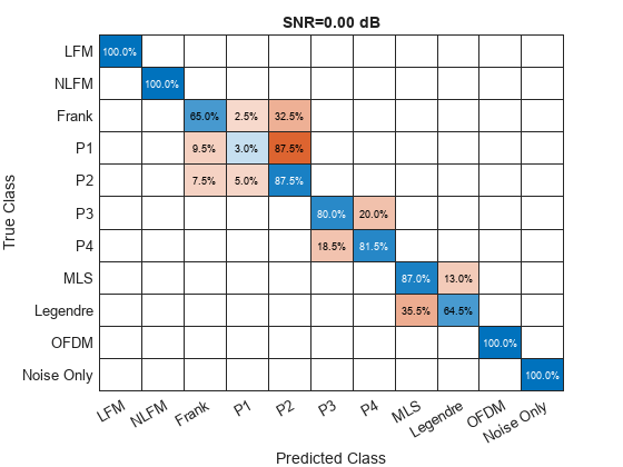
At an SNR of 0 dB, the classification performance shows a significant improvement. However, waveforms with similar time-frequency characteristics continue to exhibit a high degree of misclassification:

figure;
confusionchart(trueLabels, predictedLabels(:, 4), 'Normalization', 'row-normalized');
title(sprintf("SNR=%.2f dB", SNR(4)));

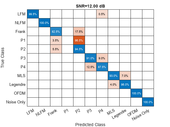
As the SNR increases to 12 dB, the network demonstrates an improved capacity to differentiate between MLS and Legendre waveforms. However, there is no improvement in differentiating P1 from P2 when compared to the results at 0 dB SNR. This persistent confusion underscores the limitations inherent in the time-frequency features extracted by the STFT and CWT for the purpose of waveform classification. For most of the remaining waveforms, the classification accuracy exceeds 90%, indicating a robust performance by the network under higher SNR conditions.

figure;
confusionchart(trueLabels, predictedLabels(:, 8), 'Normalization', 'row-normalized');
title(sprintf("SNR=%.2f dB", SNR(8)));

Conclusion

This example illustrates the process of training a time-frequency CNN for radar waveform classification. A synthetic dataset comprising ten distinct waveforms is generated, serving as the foundation for constructing and training the time-frequency CNN. The evaluation of the model's classification efficacy is conducted across varying SNR levels. Results indicate that classification accuracy can surpass 90% for certain modulation types, provided that the SNR is sufficiently high. However, the analysis reveals that at lower SNR levels, the time-frequency features, such as the STFT spectrogram and CWT scalogram, are susceptible to noise interference. Under these conditions, the classifier struggles to reliably discern the modulation characteristics of the waveforms from the time-frequency information. Moreover, waveforms with spectral characteristics resembling noise such phased-coded waveforms based on pseudo random sequences and the OFDM waveform, are prone to misclassification. Finally, waveforms with closely related modulation schemes, such as P1 and P2, are also at risk of being incorrectly classified, even in scenarios with high SNR.

References

Kong, Seung-Hyun, Minjun Kim, Linh Manh Hoang, and Eunhui Kim. "Automatic LPI radar waveform recognition using CNN." Ieee Access 6 (2018): 4207-4219.
Huang, Hui, Yi Li, Jiaoyue Liu, Dan Shen, Genshe Chen, Erik Blasch, and Khanh Pham. "LPI Waveform Recognition Using Adaptive Feature Construction and Convolutional Neural Networks." IEEE Aerospace and Electronic Systems Magazine 38, no. 4 (2023): 14-26.
Levanon, Nadav, and Eli Mozeson. Radar signals. John Wiley & Sons, 2004.