Source Localization Using Generalized Cross Correlation
This example shows how to determine the position of the source of a wideband signal using generalized cross-correlation (GCC) and triangulation. For simplicity, this example is confined to a two-dimensional scenario consisting of one source and two receiving sensor arrays. You can extend this approach to more than two sensors or sensor arrays and to three dimensions.
Introduction
Source localization differs from direction-of-arrival (DOA) estimation. DOA estimation seeks to determine only the direction of a source from a sensor. Source localization determines its position. In this example, source localization consists of two steps, the first of which is DOA estimation.
Estimate the direction of the source from each sensor array using a DOA estimation algorithm. For wideband signals, many well-known direction of arrival estimation algorithms, such as Capon's method or MUSIC, cannot be applied because they employ the phase difference between elements, making them suitable only for narrowband signals. In the wideband case, instead of phase information, you can use the difference in the signal's time-of-arrival among elements. To compute the time-of-arrival differences, this example uses the generalized cross-correlation with phase transformation (GCC-PHAT) algorithm. From the differences in time-of-arrival, you can compute the DOA. (For another example of narrowband DOA estimation algorithms, see High Resolution Direction of Arrival Estimation).
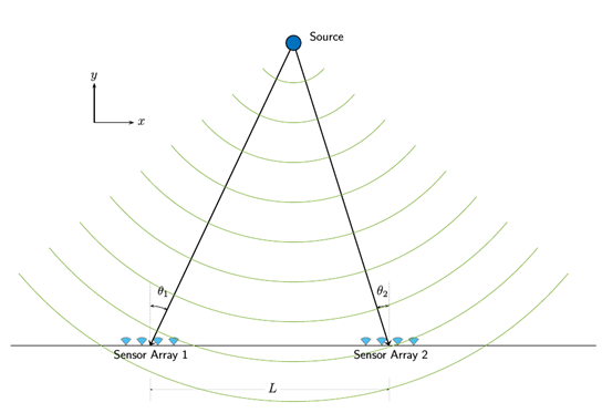
Calculate the source position by triangulation. First, draw straight lines from the arrays along the directions-of-arrival. Then, compute the intersection of these two lines. This is the source location. Source localization requires knowledge of the position and orientation of the receiving sensors or sensor arrays.
Triangulation Formula
The triangulation algorithm is based on simple trigonometric formulas. Assume that the sensor arrays are located at the 2-D coordinates (0,0) and (L,0) and the unknown source location is (x,y). From knowledge of the sensor arrays positions and the two directions-of-arrival at the arrays, and , you can compute the (x,y) coordinates from
which you can solve for y
and then for x
The remainder of this example shows how you can use the functions and System objects of the Phased Array System Toolbox™ to compute source position.
Source and Sensor Geometry
Set up two receiving 4-element ULAs aligned along the x-axis of the global coordinate system and spaced 50 meters apart. The phase center of the first array is (0,0,0). The phase center of the second array is (50,0,0). The source is located at (30,100) meters. As indicated in the figure, the receiving array gains point in the +y direction. The source transmits in the -y direction.
Specify the baseline between sensor arrays.
L = 50;
Create a 4-element receiver ULA of omnidirectional microphones. You can use the same phased.ULA System object™ for the phased.WidebandCollector and phased.GCCEstimator System objects for both arrays.
N = 4;
rxULA = phased.ULA('Element',phased.OmnidirectionalMicrophoneElement,...
    'NumElements',N);
Specify the position and orientation of the first sensor array. When you create a ULA, the array elements are automatically spaced along the y-axis. You must rotate the local axes of the array by 90° to align the elements along the x-axis of the global coordinate system.
rxpos1 = [0;0;0];
rxvel1 = [0;0;0];
rxax1 = azelaxes(90,0);
Specify the position and orientation of the second sensor array. Choose the local axes of the second array to align with the local axes of the first array.
rxpos2 = [L;0;0];
rxvel2 = [0;0;0];
rxax2 = rxax1;
Specify the signal source as a single omnidirectional transducer.
srcpos = [30;100;0];
srcvel = [0;0;0];
srcax = azelaxes(-90,0);
srcULA = phased.OmnidirectionalMicrophoneElement;
Define Waveform
Choose the source signal to be a wideband LFM waveform. Assume the operating frequency of the system is 300 kHz and set the bandwidth of the signal to 100 kHz. Assume a maximum operating range of 150 m. Then, you can set the pulse repetition interval (PRI) and the pulse repetition frequency (PRF). Assume a 10% duty cycle and set the pulse width. Finally, use a speed of sound in an underwater channel of 1500 m/s.
Set the LFM waveform parameters and create the phased.LinearFMWaveform System object.
fc = 300e3;             % 300 kHz
c = 1500;               % 1500 m/s
dmax = 150;             % 150 m
pri = (2*dmax)/c;
prf = 1/pri;
bw = 100.0e3;           % 100 kHz
fs = 2*bw;
waveform = phased.LinearFMWaveform('SampleRate',fs,'SweepBandwidth',bw,...
    'PRF',prf,'PulseWidth',pri/10);
The transmit signal can then be generated as
signal = waveform();
Radiate, Propagate, and Collect Signals
Modeling the radiation and propagation for wideband systems is more complicated than modeling narrowband systems. For example, the attenuation depends on frequency. The Doppler shift as well as the phase shifts among elements due to the signal incoming direction also vary according to the frequency. Thus, it is critical to model those behaviors when dealing with wideband signals. This example uses a subband approach.
Set the number of subbands to 128.
nfft = 128;
Specify the source radiator and the sensor array collectors.
radiator = phased.WidebandRadiator('Sensor',srcULA,...
    'PropagationSpeed',c,'SampleRate',fs,...
    'CarrierFrequency',fc,'NumSubbands',nfft);
collector1 = phased.WidebandCollector('Sensor',rxULA,...
    'PropagationSpeed',c,'SampleRate',fs,...
    'CarrierFrequency',fc,'NumSubbands',nfft);
collector2 = phased.WidebandCollector('Sensor',rxULA,...
    'PropagationSpeed',c,'SampleRate',fs,...
    'CarrierFrequency',fc,'NumSubbands',nfft);
Create the wideband signal propagators for the paths from the source to the two sensor arrays.
channel1 = phased.WidebandFreeSpace('PropagationSpeed',c,...
    'SampleRate',fs,'OperatingFrequency',fc,'NumSubbands',nfft);
channel2 = phased.WidebandFreeSpace('PropagationSpeed',c,...
    'SampleRate',fs,'OperatingFrequency',fc,'NumSubbands',nfft);
Determine the propagation directions from the source to the sensor arrays. Propagation directions are with respect to the local coordinate system of the source.
[~,ang1t] = rangeangle(rxpos1,srcpos,srcax);
[~,ang2t] = rangeangle(rxpos2,srcpos,srcax);
Radiate the signal from the source in the directions of the sensor arrays.
sigt = radiator(signal,[ang1t ang2t]);
Then, propagate the signal to the sensor arrays.
sigp1 = channel1(sigt(:,1),srcpos,rxpos1,srcvel,rxvel1);
sigp2 = channel2(sigt(:,2),srcpos,rxpos2,srcvel,rxvel2);
Compute the arrival directions of the propagated signal at the sensor arrays. Because the collector response is a function of the directions of arrival in the sensor array local coordinate system, pass the local coordinate axes matrices to the rangeangle function.
[~,ang1r] = rangeangle(srcpos,rxpos1,rxax1);
[~,ang2r] = rangeangle(srcpos,rxpos2,rxax2);
Collect the signal at the receive sensor arrays.
sigr1 = collector1(sigp1,ang1r);
sigr2 = collector2(sigp2,ang2r);
GCC Estimation and Triangulation
Create the GCC-PHAT estimators.
doa1 = phased.GCCEstimator('SensorArray',rxULA,'SampleRate',fs,...
    'PropagationSpeed',c);
doa2 = phased.GCCEstimator('SensorArray',rxULA,'SampleRate',fs,...
    'PropagationSpeed',c);
Estimate the directions of arrival.
angest1 = doa1(sigr1);
angest2 = doa2(sigr2);
Triangulate the source position using the formulas established previously. Because the scenario is confined to the x-y plane, set the z-coordinate to zero.
yest = L/(abs(tand(angest1)) + abs(tand(angest2)));
xest = yest*abs(tand(angest1));
zest = 0;
srcpos_est = [xest;yest;zest]
srcpos_est = 3×1

   29.9881
  100.5743
         0
The estimated source location matches the true location to within 30 cm.
Summary
This example showed how to perform source localization using triangulation. In particular, the example showed how to simulate, propagate, and process wideband signals. The GCC-PHAT algorithm is used to estimate the direction of arrival of a wideband signal.