Waveform Scheduling Based on Target Detection
In radar operation, it is often necessary to adjust the operation mode based on the target return. This example shows how to model a radar that changes its pulse repetition frequency (PRF) based on the radar detection.
This example requires SimEvents®.
Available Example Implementations
This example includes one Simulink® model:
Dynamic PRF Selection Based on Radar Detection: slexPRFSelectionSEExample.slx
Dynamic PRF Selection Based on Radar Detection
This model simulates a monostatic radar that searches for targets with an unambiguous range of 5 km. If the radar detects a target within 2 km, then it will switch to a higher PRF to only look for targets with 2 km range and enhance its capability to detect high speed targets.

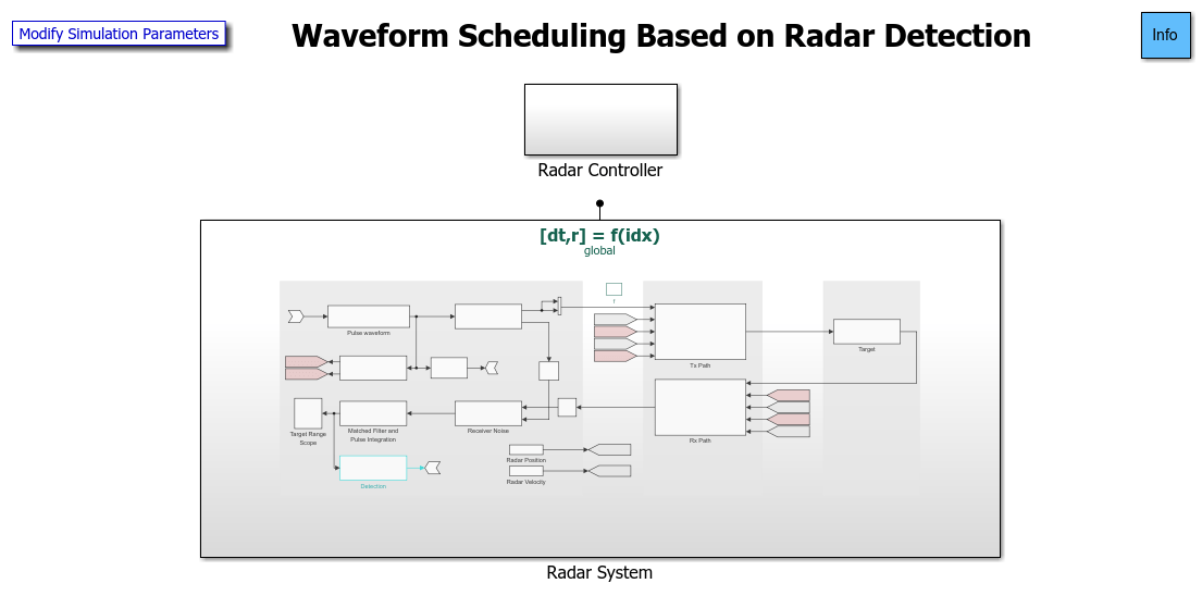
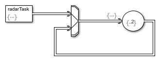
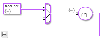
The model consists of two main subsystem, a radar system and its corresponding controller. From the top level, the radar system resides in a Simulink function block. Note that the underlying function is specified in the figure as [dt,r] = f(idx). This means that the radar takes one input, idx, which specifies the index of selected PRF of the transmitted signal and returns two outputs: dt, the time the next pulse should be transmitted and r, the detected target range of the radar system. The radar controller, shown in the following figure, uses the detection and the time to schedule when and what to transmit next.

Radar System
The radar system resides in a Simulink function block and is shown in the following figure.

The system is very similar to what is used in the Waveform Scheduling Based on Target Detection example with the following notable difference:
The waveform block is no longer a source block. Instead, it takes an input,
idx, to select which PRF to use. The available PRF values are specified in the PRF parameter of the waveform dialog.The output of the waveform is also used to compute the time,
dt, that the next pulse should be transmitted. Note that in this case, the time interval is proportional to the length of the transmitted signal.At the end of the signal processing chain, the target range is estimated and returned in
r. The controller will use this information to decide which PRF to choose for next transmission.Once the model is compiled, notice that the signal passing through the system can vary in length because of a possible change of the waveform PRF. In addition, because the sample rate cannot be derived inside a Simulink function subsystem, the sample rate is specified in the block diagrams, such as the Tx and Rx paths, the receiver preamp, and other blocks.


Exploring the Example
Several dialog parameters of the model are calculated by the helper function helperslexPRFSelectionParam. To open the function from the model, click on Modify Simulation Parameters block. This function is executed once when the model is loaded. It exports to the workspace a structure whose fields are referenced by the dialogs. To modify any parameters, either change the values in the structure at the command prompt or edit the helper function and rerun it to update the parameter structure.
Results and Displays
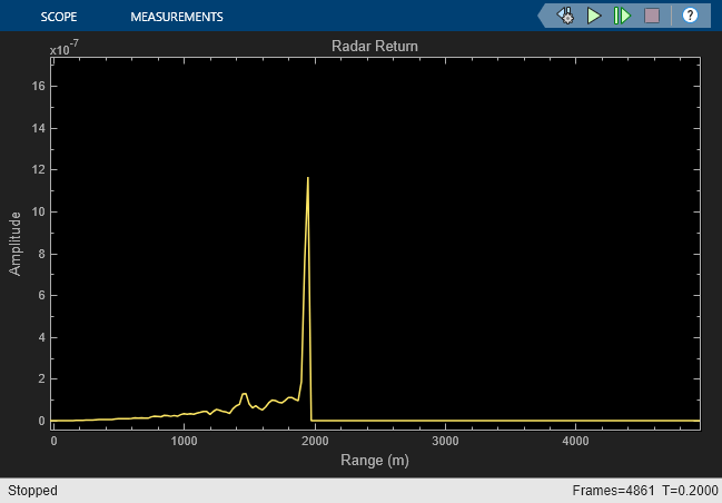
The figure below shows the detected ranges of the targets. Target ranges are computed from the round-trip time delay of the reflected signals from the targets. At the simulation start, the radar detects two targets, one is slightly over 2 km away and the other one is at approximately 3.5 km away.

After some time, the first target moves into the 2 km zone and triggers a change of PRF. Then the received signal only covers the range up to 2 km. The display is zero padded to ensure that the plot limits do not change. Notice that the target at 3.5 km gets folded to the 1.5 km range due to range ambiguity.

Summary
This example shows how to build a radar system in Simulink® that dynamically changes its PRF based on the target detection range. A staggered PRF system can be modeled similarly.