Fault Detection Using an Extended Kalman Filter
This example shows how to use an extended Kalman filter for fault detection. The example uses an extended Kalman filter for online estimation of the friction of a simple DC motor. Significant changes in the estimated friction are detected and indicate a fault. This example uses functionality from System Identification Toolbox™, and does not require Predictive Maintenance Toolbox™.
Motor Model
The motor is modeled as an inertia J with damping coefficient c, driven by a torque u. The motor angular velocity w and acceleration , are the measured outputs.
To estimate the damping coefficient c using an extended Kalman filter, introduce an auxiliary state for the damping coefficient and set its derivative to zero.
Thus, the model state, x = [w;c], and measurement, y, equations are:
The continuous-time equations are transformed to discrete time using the approximation , where Ts is the discrete sampling period. This gives the discrete-time model equations which are implemented in the pdmMotorModelStateFcn.m and pdmMotorModelMeasurementFcn.m functions.
Specify motor parameters.
J  = 10;    % Inertia
Ts = 0.01;  % Sample time
Specify initial states.
x0 = [...
    0; ...  % Angular velocity
    1];     % Friction

type pdmMotorModelStateFcn
function x1 = pdmMotorModelStateFcn(x0,varargin)
%PDMMOTORMODELSTATEFCN
%
% State update equations for a motor with friction as a state
%
%  x1 = pdmMotorModelStateFcn(x0,u,J,Ts)
%
%  Inputs:
%    x0 - initial state with elements [angular velocity; friction]
%    u  - motor torque input
%    J  - motor inertia
%    Ts - sampling time
%
%  Outputs:
%    x1 - updated states
%

%  Copyright 2016-2017 The MathWorks, Inc.

% Extract data from inputs
u  = varargin{1};   % Input
J  = varargin{2};   % System innertia
Ts = varargin{3};   % Sample time

% State update equation
x1 = [...
    x0(1)+Ts/J*(u-x0(1)*x0(2)); ...
    x0(2)];
end
type pdmMotorModelMeasurementFcnfunction y = pdmMotorModelMeasurementFcn(x,varargin)
%PDMMOTORMODELMEASUREMENTFCN
%
% Measurement equations for a motor with friction as a state
%
% y = pdmMotorModelMeasurementFcn(x0,u,J,Ts)
%
% Inputs:
% x - motor state with elements [angular velocity; friction]
% u - motor torque input
% J - motor inertia
% Ts - sampling time
%
% Outputs:
% y - motor measurements with elements [angular velocity; angular acceleration]
%
% Copyright 2016-2017 The MathWorks, Inc.
% Extract data from inputs
u = varargin{1}; % Input
J = varargin{2}; % System innertia
% Output equation
y = [...
x(1); ...
(u-x(1)*x(2))/J];
end
The motor experiences state (process) noise disturbances, q, and measurement noise disturbances, r. The noise terms are additive.
The process and measurement noise have zero mean, E[q]=E[r]=0, and covariances Q = E[qq'] and R = E[rr']. The friction state has a high process noise disturbance. This reflects the fact that we expect the friction to vary during normal operation of the motor and want the filter to track this variation. The acceleration and velocity state noise is low but the velocity and acceleration measurements are relatively noisy.
Specify the process noise covariance.
Q = [...
    1e-6 0; ...   % Angular velocity
    0 1e-2];      % Friction
Specify the measurement noise covariance.
R = [...
    1e-4 0; ...  % Velocity measurement
    0 1e-4];     % Acceleration measurement
Creating an Extended Kalman Filter
Create an extended Kalman Filter to estimate the states of the model. We are particularly interested in the damping state because dramatic changes in this state value indicate a fault event.
Create an extendedKalmanFilter object, and specify the Jacobians of the state transition and measurement functions.
ekf = extendedKalmanFilter(...
    @pdmMotorModelStateFcn, ...
    @pdmMotorModelMeasurementFcn, ...
    x0,...
    'StateCovariance',            [1 0; 0 1000], ...[1 0 0; 0 1 0; 0 0 100], ...
    'ProcessNoise',               Q, ...
    'MeasurementNoise',           R, ...
    'StateTransitionJacobianFcn', @pdmMotorModelStateJacobianFcn, ...
    'MeasurementJacobianFcn',     @pdmMotorModelMeasJacobianFcn);
The extended Kalman filter has as input arguments the state transition and measurement functions defined previously. The initial state value x0, initial state covariance, and process and measurement noise covariances are also inputs to the extended Kalman filter. In this example, the exact Jacobian functions can be derived from the state transition function f, and measurement function h:
The state Jacobian is defined in the pdmMotorModelStateJacobianFcn.m function and the measurement Jacobian is defined in the pdmMotorModelMeasJacobianFcn.m function.
type pdmMotorModelStateJacobianFcnfunction Jac = pdmMotorModelStateJacobianFcn(x,varargin)
%PDMMOTORMODELSTATEJACOBIANFCN
%
% Jacobian of motor model state equations. See pdmMotorModelStateFcn for
% the model equations.
%
% Jac = pdmMotorModelJacobianFcn(x,u,J,Ts)
%
% Inputs:
% x - state with elements [angular velocity; friction]
% u - motor torque input
% J - motor inertia
% Ts - sampling time
%
% Outputs:
% Jac - state Jacobian computed at x
%
% Copyright 2016-2017 The MathWorks, Inc.
% Model properties
J = varargin{2};
Ts = varargin{3};
% Jacobian
Jac = [...
1-Ts/J*x(2) -Ts/J*x(1); ...
0 1];
end
type pdmMotorModelMeasJacobianFcnfunction J = pdmMotorModelMeasJacobianFcn(x,varargin)
%PDMMOTORMODELMEASJACOBIANFCN
%
% Jacobian of motor model measurement equations. See
% pdmMotorModelMeasurementFcn for the model equations.
%
% Jac = pdmMotorModelMeasJacobianFcn(x,u,J,Ts)
%
% Inputs:
% x - state with elements [angular velocity; friction]
% u - motor torque input
% J - motor inertia
% Ts - sampling time
%
% Outputs:
% Jac - measurement Jacobian computed at x
%
% Copyright 2016-2017 The MathWorks, Inc.
% System parameters
J = varargin{2}; % System innertia
% Jacobian
J = [ ...
1 0;
-x(2)/J -x(1)/J];
end
Simulation
To simulate the plant, create a loop and introduce a fault in the motor (a dramatic change in the motor fiction). Within the simulation loop, use the extended Kalman filter to estimate the motor states and to specifically track the friction state to detect when there is a statistically significant change in friction.
The motor is simulated with a pulse train that repeatedly accelerates and decelerates the motor. This type of motor operation is typical for a picker robot in a production line.
t  = 0:Ts:20;                  % Time, 20s with Ts sampling period
u  = double(mod(t,1)<0.5)-0.5; % Pulse train, period 1, 50% duty cycle
nt = numel(t);                 % Number of time points
nx = size(x0,1);               % Number of states
ySig = zeros([2, nt]);         % Measured motor outputs
xSigTrue = zeros([nx, nt]);    % Unmeasured motor states
xSigEst = zeros([nx, nt]);     % Estimated motor states
xstd = zeros([nx nx nt]);      % Standard deviation of the estimated states
ySigEst = zeros([2, nt]);      % Estimated model outputs
fMean = zeros(1,nt);           % Mean estimated friction
fSTD = zeros(1,nt);            % Standard deviation of estimated friction
fKur = zeros(2,nt);            % Kurtosis of estimated friction
fChanged = false(1,nt);        % Flag indicating friction change detection
When simulating the motor, add process and measurement noise similar to the Q and R noise covariance values used when constructing the extended Kalman filter. For the friction, use a much smaller noise value because the friction is mostly constant except when the fault occurs. Artificially induce the fault during the simulation.
rng('default');
Qv = chol(Q);   % Standard deviation for process noise
Qv(end) = 1e-2; % Smaller friction noise
Rv = chol(R);   % Standard deviation for measurement noise
Simulate the model using the state update equation, and add process noise to the model states. Ten seconds into the simulation, force a change in the motor friction. Use the model measurement function to simulate the motor sensors, and add measurement noise to the model outputs.
for ct = 1:numel(t)

   % Model output update
   y = pdmMotorModelMeasurementFcn(x0,u(ct),J,Ts);
   y = y+Rv*randn(2,1);   % Add measurement noise
   ySig(:,ct) = y;

   % Model state update
   xSigTrue(:,ct) = x0;
   x1 = pdmMotorModelStateFcn(x0,u(ct),J,Ts);
   % Induce change in friction
   if t(ct) == 10
       x1(2) = 10;  % Step change
   end
   x1n = x1+Qv*randn(nx,1);  % Add process noise
   x1n(2) = max(x1n(2),0.1); % Lower limit on friction
   x0 = x1n; % Store state for next simulation iteration
To estimate the motor states from the motor measurements, use the predict and correct commands of the extended Kalman Filter.
   % State estimation using the Extended Kalman Filter
   x_corr = correct(ekf,y,u(ct),J,Ts); % Correct the state estimate based on current measurement.
   xSigEst(:,ct) = x_corr;
   xstd(:,:,ct) = chol(ekf.StateCovariance);
   predict(ekf,u(ct),J,Ts);            % Predict next state given the current state and input.
To detect changes in friction, compute the estimated friction mean and standard deviation using a 4 second moving window. After an initial 7-second period, lock the computed mean and standard deviation. This initially computed mean is the expected no-fault mean value for the friction. After 7 seconds, if the estimated friction is greater than 3 standard deviations away from the expected no-fault mean value, it signifies a significant change in the friction. To reduce the effect of noise and variability in the estimated friction, use the mean of the estimated friction when comparing to the 3-standard-deviations bound.
   if t(ct) < 7
       % Compute mean and standard deviation of estimated fiction.
       idx = max(1,ct-400):max(1,ct-1); % Ts = 0.01 seconds
       fMean(ct) = mean( xSigEst(2, idx) );
       fSTD(ct)  = std( xSigEst(2, idx) );
   else
       % Store the computed mean and standard deviation without
       % recomputing.
       fMean(ct) = fMean(ct-1);
       fSTD(ct)  = fSTD(ct-1);
       % Use the expected friction mean and standard deviation to detect
       % friction changes.
       estFriction = mean(xSigEst(2,max(1,ct-10):ct));
       fChanged(ct) = (estFriction > fMean(ct)+3*fSTD(ct)) || (estFriction < fMean(ct)-3*fSTD(ct));
   end
   if fChanged(ct) && ~fChanged(ct-1)
       % Detect a rising edge in the friction change signal |fChanged|.
       fprintf('Significant friction change at %f\n',t(ct));
   end
Significant friction change at 10.450000
Use the estimated state to compute the estimated output. Compute the error between the measured and estimated outputs, and calculate the error statistics. The error statistics can be used for detecting the friction change. This is discussed in more detail later.
   ySigEst(:,ct) = pdmMotorModelMeasurementFcn(x_corr,u(ct),J,Ts);
   idx = max(1,ct-400):ct;
   fKur(:,ct) = [...
       kurtosis(ySigEst(1,idx)-ySig(1,idx)); ...
       kurtosis(ySigEst(2,idx)-ySig(2,idx))];
end
Extended Kalman Filter Performance
Note that a friction change was detected at 10.45 seconds. We now describe how this fault-detection rule was derived. First examine the simulation results and filter performance.
figure,
subplot(211), plot(t,ySig(1,:),t,ySig(2,:));
title('Motor Outputs')
legend('Measured Angular Velocity','Measured Angular Acceleration', 'Location','SouthWest')
subplot(212), plot(t,u);
title('Motor Input - Torque')
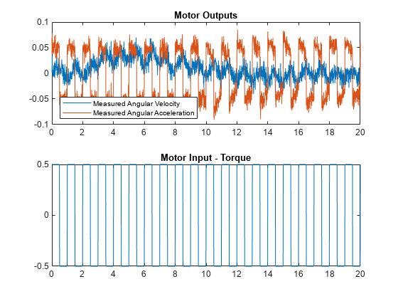
The model input-output responses indicate that it is difficult to detect the friction change directly from the measured signals. The extended Kalman filter enables us to estimate the states, in particular the friction state. Compare the true model states and estimated states. The estimated states are shown with confidence intervals corresponding to 3 standard deviations.
figure,
subplot(211),plot(t,xSigTrue(1,:), t,xSigEst(1,:), ...
    [t nan t],[xSigEst(1,:)+3*squeeze(xstd(1,1,:))', nan, xSigEst(1,:)-3*squeeze(xstd(1,1,:))'])
axis([0 20 -0.06 0.06]),
legend('True value','Estimated value','Confidence interval')
title('Motor State - Velocity')
subplot(212),plot(t,xSigTrue(2,:), t,xSigEst(2,:),  ...
    [t nan t],[xSigEst(2,:)+3*squeeze(xstd(2,2,:))' nan xSigEst(2,:)-3*squeeze(xstd(2,2,:))'])
axis([0 20 -10 15])
title('Motor State - Friction');
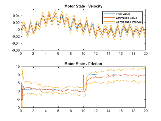
Note that the filter estimate tracks the true values, and that the confidence intervals remain bounded. Examining the estimation errors provide more insight into the filter behavior.
figure,
subplot(211),plot(t,xSigTrue(1,:)-xSigEst(1,:))
title('Velocity State Error')
subplot(212),plot(t,xSigTrue(2,:)-xSigEst(2,:))
title('Friction State Error')
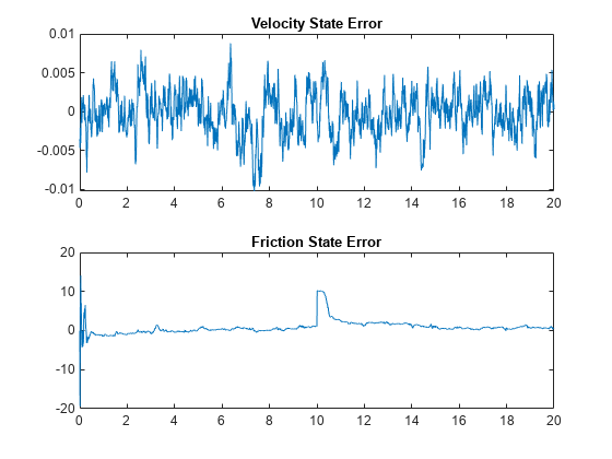
The error plots show that the filter adapts after the friction change at 10 seconds and reduces the estimation errors to zero. However, the error plots cannot be used for fault detection as they rely on knowing the true states. Comparing the measured state value to the estimated state values for acceleration and velocity could provide a detection mechanism.
figure
subplot(211), plot(t,ySig(1,:)-ySigEst(1,:))
title('Velocity Measurement Error')
subplot(212),plot(t,ySig(2,:)-ySigEst(2,:))
title('Acceleration Measurement Error')
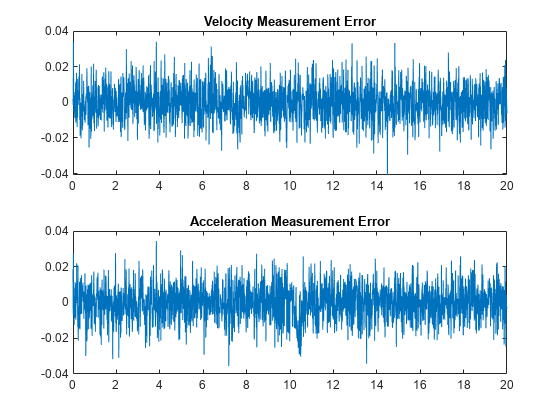
The acceleration error plot shows a minor difference in mean error around 10 seconds when the fault is introduced. View the error statistics to see if the fault can be detected from the computed errors. The acceleration and velocity errors are expected to be normally distributed (the noise models are all Gaussian). Therefore, the kurtosis of the acceleration error may help identify when the error distribution change from symmetrical to asymmetrical due to the friction change and resulting change in error distribution.
figure,
subplot(211),plot(t,fKur(1,:))
title('Velocity Error Kurtosis')
subplot(212),plot(t,fKur(2,:))
title('Acceleration Error Kurtosis')
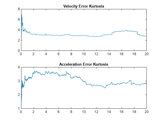
Ignoring the first 4 seconds when the estimator is still converging and data is being collected, the kurtosis of the errors is relatively constant with minor variations around 3 (the expected kurtosis value for a Gaussian distribution). Thus, the error statistics cannot be used to automatically detect friction changes in this application. Using the kurtosis of the errors is also difficult in this application as the filter is adapting and continually driving the errors to zero, only giving a short time window where the error distributions differ from zero.
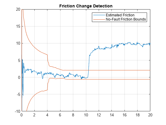
Thus in this application, using the changes in estimated friction provide the best way to automatically detect faults in the motor. The friction estimates (mean and standard deviation) from known no-fault data provide expected bounds for the friction and it is easy to detect when these bounds are violated. The following plot highlights this fault-detection approach.
figure
plot(t,xSigEst(2,:),[t nan t],[fMean+3*fSTD,nan,fMean-3*fSTD])
title('Friction Change Detection')
legend('Estimated Friction','No-Fault Friction Bounds')
axis([0 20 -10 20])
grid on
Summary
This example has shown how to use an extended Kalman filter to estimate the friction in a simple DC motor and use the friction estimate for fault detection.