Fault Diagnosis of Centrifugal Pumps Using Residual Analysis

This example uses:

This example shows a model parity-equations based approach for detection and diagnosis of different types of faults that occur in a pumping system. This example extends the techniques presented in the Fault Diagnosis of Centrifugal Pumps Using Steady State Experiments to the situation where the pump operation spans multiple operating conditions.

The example follows the centrifugal pump analysis presented in the Fault Diagnosis Applications book by Rolf Isermann [1]. It uses functionality from System Identification Toolbox™, Statistics and Machine Learning Toolbox™, Control System Toolbox™ and Simulink™ and does not require Predictive Maintenance Toolbox™.

Multi-Speed Pump Runs - Diagnosis by Residual Analysis

The steady-state pump head and torque equations do not produce accurate results if the pump is run at rapidly varying or a wider range of speeds. Friction and other losses could become significant and the model's parameters exhibit dependence on speed. A widely applicable approach in such cases is to create a black box model of the behavior. The parameters of such models need not be physically meaningful. The model is used as a device for simulation of known behaviors. The model's outputs are subtracted from the corresponding measured signals to compute residuals. The properties of residuals, such as their mean, variance and power are used to distinguish between normal and faulty operations.

Using the static pump head equation, and the dynamic pump-pipe equations, the 4 residuals as shown in the figure can be computed.

The model has of the following components:

Static pump model: $Δ p_{}^{ˆ} (t) = θ_{1} ω^{2} (t) + θ_{2} ω (t)$
Dynamic pipe model: $Q_{}^{ˆ} (t) = θ_{3} + θ_{4} \sqrt{Δ p (t)} + θ_{5} Q_{}^{ˆ} (t - 1)$
Dynamic pump-pipe model: ${Q_{}^{ˆ}}_{}^{ˆ} (t) = θ_{3} + θ_{4} \sqrt{{Δ p (t)}_{}^{ˆ}} + θ_{5} {Q_{}^{ˆ}}_{}^{ˆ} (t - 1)$
Dynamic inverse pump model: ${M_{}^{ˆ}}_{m o t o r} (t) = θ_{6} + θ_{7} ω (t) + θ_{8} ω (t - 1) + θ_{9} ω^{2} (t) + θ_{10} {M_{}^{ˆ}}_{m o t o r} (t - 1)$

The model parameters $θ_{1}, . . ., θ_{10}$ show dependence on pump speed. In this example, a piecewise linear approximation for the parameters is computed. Divide the operating region into 3 regimes:

$ω \leq 900 R P M$
$900 < ω \leq 1500 R P M$
$ω > 1500 R P M$

A healthy pump was run over a reference speed range of 0 - 3000 RPM in closed loop with a closed-loop controller. The reference input is a modified PRBS signal. The measurements for motor torque, pump torque, speed and pressure were collected at 10 Hz sampling frequency. Load the measured signals and plot the reference and actual pump speeds (these are large datasets, ~20MB, that are downloaded from the MathWorks support files site).

url = 'https://www.mathworks.com/supportfiles/predmaint/fault-diagnosis-of-centrifugal-pumps-using-residual-analysis/DynamicOperationData.mat';
websave('DynamicOperationData.mat',url);
load DynamicOperationData
figure
plot(t, RefSpeed, t, w)
xlabel('Time (s)')
ylabel('Pump Speed (RPM)')
legend('Reference','Actual')

Define operating regimes based on pump speed ranges.

I1 = w<=900;            % first operating regime
I2 = w>900 & w<=1500;   % second operating regime
I3 = w>1500;            % third operating regime

Model Identification

A. Static Pump Model Identification

Estimate the parameters $θ_{1}$ and $θ_{2}$ in the static pump equation using the measured values of pump speed $ω (t)$ and pressure differential $Δ p (t)$ as input-output data. See the helper function staticPumpEst that performs this estimation.

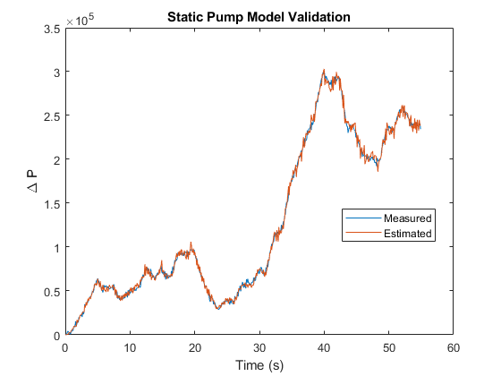
th1 = zeros(3,1);  
th2 = zeros(3,1); 
dpest = nan(size(dp));  % estimated pressure difference
[th1(1), th2(1), dpest(I1)] = staticPumpEst(w, dp, I1);  % Theta1, Theta2 estimates for regime 1
[th1(2), th2(2), dpest(I2)] = staticPumpEst(w, dp, I2);  % Theta1, Theta2 estimates for regime 2
[th1(3), th2(3), dpest(I3)] = staticPumpEst(w, dp, I3);  % Theta1, Theta2 estimates for regime 3
plot(t, dp, t, dpest) % compare measured and predicted pressure differential
xlabel('Time (s)')
ylabel('\Delta P')
legend('Measured','Estimated','Location','best')
title('Static Pump Model Validation')

B. Dynamic Pipe Model Identification

Estimate the parameters $θ_{3}$ , $θ_{4}$ and $θ_{5}$ in the pipe discharge flow equation $Q_{}^{ˆ} (t) = θ_{3} + θ_{4} \sqrt{Δ p (t)} + θ_{5} Q_{}^{ˆ} (t - 1)$ , using the measured values of flow rate $Q (t)$ and pressure differential $Δ p (t)$ as input-output data. See the helper function dynamicPipeEst that performs this estimation.

th3 = zeros(3,1);  
th4 = zeros(3,1); 
th5 = zeros(3,1);
[th3(1), th4(1), th5(1)] = dynamicPipeEst(dp, Q, I1); % Theta3, Theta4, Theta5 estimates for regime 1
[th3(2), th4(2), th5(2)] = dynamicPipeEst(dp, Q, I2); % Theta3, Theta4, Theta5 estimates for regime 2
[th3(3), th4(3), th5(3)] = dynamicPipeEst(dp, Q, I3); % Theta3, Theta4, Theta5 estimates for regime 3

Unlike the static pump model case, the dynamic pipe model shows dynamic dependence on flow rate values. To simulate the model under varying speed regimes, a piecewise-linear model is created in Simulink using the "LPV System" block of Control System Toolbox. See the Simulink model LPV_pump_pipe and the helper function simulatePumpPipeModel that performs the simulation.

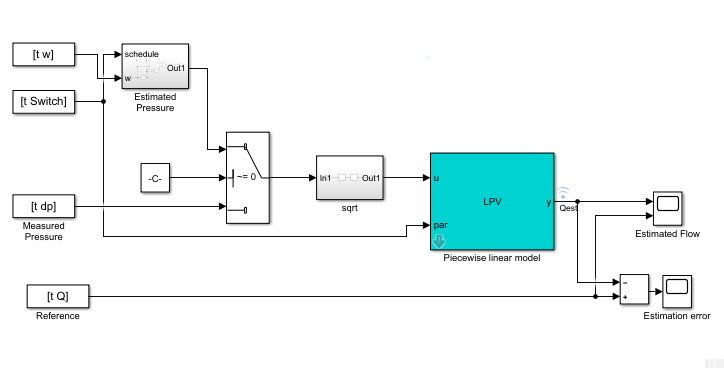
% Check Control System Toolbox availability
ControlsToolboxAvailable = ~isempty(ver('control')) && license('test', 'Control_Toolbox');
if ControlsToolboxAvailable
    % Simulate the dynamic pipe model. Use measured value of pressure as input
    Ts = t(2)-t(1);
    Switch = ones(size(w));
    Switch(I2) = 2;
    Switch(I3) = 3;
    UseEstimatedP = 0;
    Qest_pipe = simulatePumpPipeModel(Ts,th3,th4,th5);
    plot(t,Q,t,Qest_pipe) % compare measured and predicted flow rates
else
    % Load pre-saved simulation results from the piecewise linear Simulink model
    load DynamicOperationData Qest_pipe
    Ts = t(2)-t(1);
    plot(t,Q,t,Qest_pipe)
end
xlabel('Time (s)')
ylabel('Flow rate (Q), m^3/s')
legend('Measured','Estimated','Location','best')
title('Dynamic Pipe Model Validation')

C. Dynamic Pump Pipe Model Identification

The Dynamic pump-pipe model uses the same parameters identified above ( $θ_{3}, θ_{4}, θ_{5}$ ) except that the model simulation requires the use of estimated pressure difference rather than the measured one. Hence no new identification is required. Check that the estimated values of $θ_{3}, θ_{4}, θ_{5}$ give a good reproduction of the pump-pipe dynamics.

if ControlsToolboxAvailable
    UseEstimatedP = 1;
    Qest_pump_pipe = simulatePumpPipeModel(Ts,th3,th4,th5);
    plot(t,Q,t,Qest_pump_pipe) % compare measured and predicted flow rates
else
    load DynamicOperationData Qest_pump_pipe 
    plot(t,Q,t,Qest_pump_pipe)
end

xlabel('Time (s)')
ylabel('Flow rate Q (m^3/s)')
legend('Measured','Estimated','location','best')
title('Dynamic Pump-Pipe Model Validation')

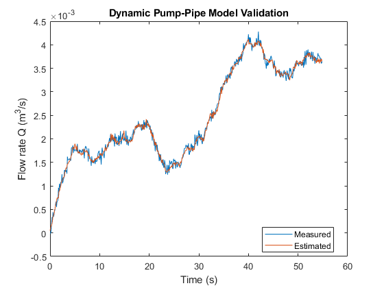
The fit is virtually identical to the one obtained using measured pressure values.

D. Dynamic Inverse Pump Model Identification

The parameters $θ_{6}, . . ., θ_{10}$ can be identified in a similar manner, by regressing the measured torque values on the previous torque and speed measurements. However, a complete multi-speed simulation of the resulting piecewise linear model does not provide a good fit to the data. Hence a different black box modeling approach is tried which involves identifying a Nonlinear ARX model with rational regressors to fit the data.

% Use first 300 samples out of 550 for identification
N = 350;
sys3 = identifyNonlinearARXModel(Mmot,w,Q,Ts,N)

sys3 = 
Nonlinear ARX model with 1 output and 2 inputs
  Inputs: u1, u2
  Outputs: y1

Regressors:
  1. Linear regressors in variables y1, u1, u2
  2. Custom regressor: u1(t-2)^2
  3. Custom regressor: u1(t)*u2(t-2)
  4. Custom regressor: u2(t)^2
  List of all regressors

Output function: Linear Function
Sample time: 0.1 seconds

Status:                                         
Estimated using NLARX on time domain data.      
Fit to estimation data: 49.2% (simulation focus)
FPE: 1798, MSE: 3392

Mmot_est = sim(sys3,[w Q]);
plot(t,Mmot,t,Mmot_est) % compare measured and predicted motor torque
xlabel('Time (s)')
ylabel('Motor Torque (Nm)')
legend('Measured','Estimated','location','best')
title('Inverse pump model validation')

Residue Generation

Define residue of a model as the difference between a measured signal and the corresponding model-produced output. Compute the four residuals corresponding to the four model components.

r1 = dp - dpest;
r2 = Q - Qest_pipe;
r3 = Q - Qest_pump_pipe;

For computing the inverse pump model residue, apply a smoothing operation on the model output using a moving average filter since the original residues show large variance.

r4 = Mmot - movmean(Mmot_est,[1 5]);

A view of training residues:

figure
subplot(221)
plot(t,r1)
ylabel('Static pump - r1')
subplot(222)
plot(t,r2)
ylabel('Dynamic pipe - r2')
subplot(223)
plot(t,r3)
ylabel('Dynamic pump-pipe - r3')
xlabel('Time (s)')
subplot(224)
plot(t,r4)
ylabel('Dynamic inverse pump - r4')
xlabel('Time (s)')

Residue Feature Extraction

Residues are signals from which suitable features are extracted for fault isolation. Since no parametric information is available, consider features that are derived purely from signal properties such as maximum amplitude or variance of the signal.

Consider a set of 20 experiments on the pump-pipe system using PRBS input realizations. The experiment set is repeated for each of the following modes:

Healthy pump
Fault 1: Wear at clearance gap
Fault 2: Small deposits at impeller outlet
Fault 3: Deposits at impeller inlet
Fault 4: Abrasive wear at impeller outlet
Fault 5: Broken blade
Fault 6: Cavitation
Fault 7: Speed sensor bias
Fault 8: Flowmeter bias
Fault 9: Pressure sensor bias

Load the experimental data

url = 'https://www.mathworks.com/supportfiles/predmaint/fault-diagnosis-of-centrifugal-pumps-using-residual-analysis/MultiSpeedOperationData.mat';
websave('MultiSpeedOperationData.mat',url);
load MultiSpeedOperationData
% Generate operation mode labels
Labels = {'Healthy','ClearanceGapWear','ImpellerOutletDeposit',...
    'ImpellerInletDeposit','AbrasiveWear','BrokenBlade','Cavitation','SpeedSensorBias',...
    'FlowmeterBias','PressureSensorBias'};

Compute residues for each ensemble and each mode of operation. This takes several minutes. Hence the residual data is saved in a data file. Run the helperComputeEnsembleResidues to generate the residuals, as in:

% HealthyR = helperComputeEnsembleResidues(HealthyEnsemble,Ts,sys3,th1,th2,th3,th4,th5); % Healthy data residuals

% Load pre-saved data from "helperComputeEnsembleResidues" run
url = 'https://www.mathworks.com/supportfiles/predmaint/fault-diagnosis-of-centrifugal-pumps-using-residual-analysis/Residuals.mat';
websave('Residuals.mat',url);
load Residuals

The feature of the residues that would have the most mode-discrimination power is not known a-priori. So generate several candidate features: mean, maximum amplitude, variance, kurtosis and 1-norm for each residual. All the features are scaled using the range of values in the healthy ensemble.

CandidateFeatures = {@mean, @(x)max(abs(x)), @kurtosis, @var, @(x)sum(abs(x))};
FeatureNames = {'Mean','Max','Kurtosis','Variance','OneNorm'};
% generate feature table from gathered residuals of each fault mode
[HealthyFeature, MinMax] = helperGenerateFeatureTable(HealthyR, CandidateFeatures, FeatureNames);
Fault1Feature  = helperGenerateFeatureTable(Fault1R,  CandidateFeatures, FeatureNames, MinMax);
Fault2Feature  = helperGenerateFeatureTable(Fault2R,  CandidateFeatures, FeatureNames, MinMax);
Fault3Feature  = helperGenerateFeatureTable(Fault3R,  CandidateFeatures, FeatureNames, MinMax);
Fault4Feature  = helperGenerateFeatureTable(Fault4R,  CandidateFeatures, FeatureNames, MinMax);
Fault5Feature  = helperGenerateFeatureTable(Fault5R,  CandidateFeatures, FeatureNames, MinMax);
Fault6Feature  = helperGenerateFeatureTable(Fault6R,  CandidateFeatures, FeatureNames, MinMax);
Fault7Feature  = helperGenerateFeatureTable(Fault7R,  CandidateFeatures, FeatureNames, MinMax);
Fault8Feature  = helperGenerateFeatureTable(Fault8R,  CandidateFeatures, FeatureNames, MinMax);
Fault9Feature  = helperGenerateFeatureTable(Fault9R,  CandidateFeatures, FeatureNames, MinMax);

There are 20 features in each feature table (5 features for each residue signal). Each table contains 50 observations (rows), one from each experiment.

N = 50; % number of experiments in each mode
FeatureTable = [...
   [HealthyFeature(1:N,:), repmat(Labels(1),[N,1])];...
   [Fault1Feature(1:N,:),  repmat(Labels(2),[N,1])];...
   [Fault2Feature(1:N,:),  repmat(Labels(3),[N,1])];...
   [Fault3Feature(1:N,:),  repmat(Labels(4),[N,1])];...
   [Fault4Feature(1:N,:),  repmat(Labels(5),[N,1])];...
   [Fault5Feature(1:N,:),  repmat(Labels(6),[N,1])];...
   [Fault6Feature(1:N,:),  repmat(Labels(7),[N,1])];...
   [Fault7Feature(1:N,:),  repmat(Labels(8),[N,1])];...
   [Fault8Feature(1:N,:),  repmat(Labels(9),[N,1])];...
   [Fault9Feature(1:N,:),  repmat(Labels(10),[N,1])]];
FeatureTable.Properties.VariableNames{end} = 'Condition';

% Preview some samples of training data
disp(FeatureTable([2 13 37 49 61 62 73 85 102 120],:))

     Mean1       Mean2      Mean3      Mean4      Max1        Max2        Max3        Max4       Kurtosis1    Kurtosis2    Kurtosis3    Kurtosis4     Variance1    Variance2    Variance3    Variance4    OneNorm1    OneNorm2    OneNorm3    OneNorm4            Condition        
    ________    _______    _______    _______    _______    ________    ________    _________    _________    _________    _________    __________    _________    _________    _________    _________    ________    ________    ________    ________    _________________________

     0.32049     0.6358     0.6358    0.74287    0.39187     0.53219     0.53219     0.041795      0.18957    0.089492     0.089489              0     0.45647       0.6263       0.6263      0.15642      0.56001    0.63541     0.63541      0.24258    {'Healthy'              }
     0.21975    0.19422    0.19422    0.83704          0     0.12761     0.12761      0.27644      0.18243     0.19644      0.19643        0.20856    0.033063      0.16772      0.16773     0.025119     0.057182    0.19344     0.19344     0.063167    {'Healthy'              }
      0.1847    0.25136    0.25136    0.87975    0.32545     0.13929      0.1393     0.084162      0.72346    0.091488     0.091485       0.052552    0.063757      0.18371      0.18371     0.023845      0.10671    0.25065     0.25065      0.04848    {'Healthy'              }
           1          1          1          0    0.78284     0.94535     0.94535       0.9287      0.41371     0.45927      0.45926        0.75934     0.92332            1            1      0.80689      0.99783          1           1       0.9574    {'Healthy'              }
     -2.6545    0.90555    0.90555    0.86324     1.3037      0.7492      0.7492      0.97823    -0.055035     0.57019      0.57018         1.4412      1.4411      0.73128      0.73128      0.80573       3.2084    0.90542     0.90542      0.49257    {'ClearanceGapWear'     }
    -0.89435    0.43384    0.43385     1.0744    0.82197     0.30254     0.30254    -0.022325      0.21411    0.098504       0.0985      -0.010587     0.55959      0.29554      0.29554     0.066693       1.0432    0.43326     0.43326      0.13785    {'ClearanceGapWear'     }
     -1.2149    0.53579    0.53579     1.0899    0.87439     0.47339     0.47339      0.29547     0.058946    0.048138     0.048137        0.17864     0.79648      0.48658      0.48658      0.25686       1.4066     0.5353      0.5353      0.26663    {'ClearanceGapWear'     }
     -1.0949    0.44616    0.44616      1.143    0.56693     0.19719     0.19719    -0.012055     -0.10819     0.32603      0.32603     -0.0033592     0.43341      0.12857      0.12857     0.038392       1.2238    0.44574     0.44574     0.093243    {'ClearanceGapWear'     }
     -0.1844    0.16651    0.16651    0.87747    0.25597    0.080265    0.080265      0.49715       0.5019     0.29939      0.29938         0.5338    0.072397     0.058024     0.058025       0.1453      0.20263    0.16566     0.16566      0.14216    {'ImpellerOutletDeposit'}
     -3.0312     0.9786     0.9786    0.75241      1.473     0.97839     0.97839       1.0343    0.0050647      0.4917       0.4917        0.89759      1.7529       0.9568       0.9568       0.8869       3.6536    0.97859     0.97859      0.62706    {'ImpellerOutletDeposit'}

Classifier Design

A. Visualizing mode separability using scatter plot

Begin the analysis by visual inspection of the features. For this, consider Fault 1: Wear at clearance gap. To view which features are most suitable to detect this fault, generate a scatter plot of features with labels 'Healthy' and 'ClearanceGapWear'.

T = FeatureTable(:,1:20);
P = T.Variables;
R = FeatureTable.Condition;
I = strcmp(R,'Healthy') | strcmp(R,'ClearanceGapWear');
f = figure;
gplotmatrix(P(I,:),[],R(I))
f.Position(3:4) = f.Position(3:4)*1.5;

Although not clearly visible, features in columns 1 and 17 provide the most separation. Analyze these features more closely.

f = figure;
Names = FeatureTable.Properties.VariableNames;
J = [1 17];
fprintf('Selected features for clearance gap fault: %s\n',strjoin(Names(J),', '))

Selected features for clearance gap fault: Mean1, OneNorm1

gplotmatrix(P(I,[1 17]),[],R(I))

The plot now clearly shows that features Mean1 and OneNorm1 can be used to separate healthy mode from clearance gap fault mode. A similar analysis can be performed for each fault mode. In all cases, it is possible to find a set of features that distinguish the fault modes. Hence detection of a faulty behavior is always possible. However, fault isolation is more difficult since the same features are affected by multiple fault types. For example, the features Mean1 (Mean of r1) and OneNorm1 (1-norm of r1) show a change for many fault types. Still some faults such as sensor biases are more easily isolable where the fault is separable in many features.

For the three sensor bias faults, pick features from a manual inspection of the scatter plot.

figure;
I = strcmp(R,'Healthy') | strcmp(R,'PressureSensorBias') | strcmp(R,'SpeedSensorBias') | strcmp(R,'FlowmeterBias');
J = [1 4 6 16 20]; % selected feature indices
fprintf('Selected features for sensors'' bias: %s\n',strjoin(Names(J),', '))

Selected features for sensors' bias: Mean1, Mean4, Max2, Variance4, OneNorm4

gplotmatrix(P(I,J),[],R(I))

The scatter plot of selected features shows that the 4 modes can be distinguished on one or more pairs of features. Train a 20 member Tree Bagger classifier for the reduced set of faults (sensor biases only) using a reduced set of features.

rng default % for reproducibility
Mdl = TreeBagger(20, FeatureTable(I,[J 21]), 'Condition',...
   'OOBPrediction','on',...
   'OOBPredictorImportance','on');
figure
plot(oobError(Mdl))
xlabel('Number of trees')
ylabel('Misclassification probability')

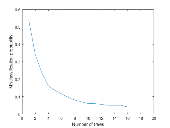
The misclassification error is less than 3%. Thus it is possible to pick and work with a smaller set of features for classifying a certain subset of faults.

B. Multi-class Classification using Classification Learner App

The previous section focused on manual inspection of scatter plots to reduce the feature set for particular fault types. This approach can get tedious and may not cover all fault types. Can you design a classifier that can handle all fault modes in a more automated fashion? There are many classifiers available in Statistics and Machine Learning Toolbox. A quick way to try many of them and compare their performances is to use the Classification Learner App.

Launch the Classification Learner App and select FeatureTable from workspace as working data for a new session. Set aside 20% of data (10 samples of each mode) for holdout validation.
Select All under Model Type section of the main tab. Then press the Train button.
In a short time, about 20 classifiers are trained. Their accuracies are displayed next to their names under the history panel. A linear SVM classifier performs the best, producing 86% accuracy on the hold out samples. This classifier has some difficulty in identifying "ClearanceGapWear" which it classifies as "ImpellerOutletDeposit" 40% of the time.
To get a graphical view of the performance, open a Confusion Matrix plot from the PLOTS section of the main tab. The plot shows the performance of the selected classifier (the Linear SVM classifier here).

Export the best performing classifier to the workspace and use it for prediction on new measurements.

Summary

A well designed fault diagnosis strategy can save operating costs by minimizing service downtime and component replacement costs. The strategy benefits from a good knowledge about the operating machine's dynamics which is used in combination with sensor measurements to detect and isolate different kinds of faults. This example described a residual based approach for fault diagnosis of centrifugal pumps. This approach is a good alternative to parameter estimation and tracking based approaches when the modeling task is complex and model parameters show dependence on operating conditions.

A residual based fault diagnosis approach involves the following steps:

Model the dynamics between the measurable inputs and outputs of the system using physical considerations or black box system identification techniques.
Compute residues as difference between measured and model produced signals. The residues may need to be further filtered to improve fault isolability.
Extract features such as peak amplitude, power, kurtosis etc from each residual signal.
Use features for fault detection and classification using anomaly detection and classification techniques.
Not all residues and derived features are sensitive to every fault. A view of feature histograms and scatter plots can reveal which features are suitable for detecting a certain fault type. This process of picking features and assessing their performance for fault isolation can be an iterative procedure.

References

Isermann, Rolf, Fault-Diagnosis Applications. Model-Based Condition Monitoring: Actuators, Drives, Machinery, Plants, Sensors, and Fault-tolerant System, Edition 1, Springer-Verlag Berlin Heidelberg, 2011.

Supporting Functions

Static pump equation parameter estimation

function [x1, x2, dpest] = staticPumpEst(w, dp, I)
%staticPumpEst Static pump parameter estimation in a varying speed setting
% I: sample indices for the selected operating region.

w1 = [0; w(I)];
dp1 = [0; dp(I)];
R1 = [w1.^2 w1];
x = pinv(R1)*dp1;
x1 = x(1);  
x2 = x(2);  

dpest = R1(2:end,:)*x;
end

Dynamic pipe parameter estimation

function [x3, x4, x5, Qest] = dynamicPipeEst(dp, Q, I)
%dynamicPipeEst Dynamic pipe parameter estimation in a varying speed setting
% I: sample indices for the selected operating region.

Q = Q(I);
dp = dp(I);
R1 = [0; Q(1:end-1)];
R2 = dp; R2(R2<0) = 0; R2 = sqrt(R2);
R = [ones(size(R2)), R2, R1];

% Remove out-of-regime samples
ii = find(I);
j = find(diff(ii)~=1);
R = R(2:end,:); R(j,:) = [];
y = Q(2:end); y(j) = [];
x = R\y;

x3 = x(1);
x4 = x(2);
x5 = x(3);

Qest = R*x;
end

Dynamic, multi-operating mode simulation of pump-pipe model using LPV System block.

function Qest = simulatePumpPipeModel(Ts,th3,th4,th5)
%simulatePumpPipeModel Piecewise linear modeling of dynamic pipe system.
% Ts: sample time
% w: Pump rotational speed
% th1, th2, th3 are estimated model parameters for the 3 regimes.
% This function requires Control System Toolbox.

ss1 = ss(th5(1),th4(1),th5(1),th4(1),Ts);
ss2 = ss(th5(2),th4(2),th5(2),th4(2),Ts);
ss3 = ss(th5(3),th4(3),th5(3),th4(3),Ts);
offset = permute([th3(1),th3(2),th3(3)]',[3 2 1]);
OP = struct('Region',[1 2 3]');
sys = cat(3,ss1,ss2,ss3);
sys.SamplingGrid = OP;

assignin('base','sys',sys)
assignin('base','offset',offset)
mdl = 'LPV_pump_pipe';
sim(mdl);
Qest = logsout.get('Qest');
Qest = Qest.Values;
Qest = Qest.Data;
end

Identify a dynamic model for inverse pump dynamics.

function syse = identifyNonlinearARXModel(Mmot,w,Q,Ts,N)
%identifyNonlinearARXModel Identify a nonlinear ARX model for 2-input (w, Q), 1-output (Mmot) data.
% Inputs:
%  w: rotational speed
%  Q: Flow rate
%  Mmot: motor torque
%  N: number of data samples to use
% Outputs:
%  syse: Identified model
%
% This function uses NLARX estimator from System Identification Toolbox.

sys = idnlarx([2 2 1 0 1],'','CustomRegressors',{'u1(t-2)^2','u1(t)*u2(t-2)','u2(t)^2'});
data = iddata(Mmot,[w Q],Ts);
opt = nlarxOptions;
opt.Focus = 'simulation';
opt.SearchOptions.MaxIterations = 500;
syse = nlarx(data(1:N),sys,opt);
end