Fault Diagnosis of Centrifugal Pumps Using Steady State Experiments

Pump Supervision and Fault Detection

Pumps are essential equipment in many industries including power and chemical, mineral and mining, manufacturing, heating, air conditioning and cooling. Centrifugal pumps are used to transport fluids by the conversion of rotational kinetic energy to the hydrodynamic energy of the fluid flow. The rotational energy typically comes from a combustion engine or electric motor. The fluid enters the pump impeller along or near to the rotating axis and is accelerated by the impeller, flowing radially outward into a diffuser.

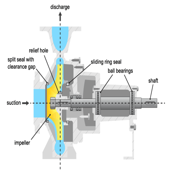
Pumps experience damage to their hydraulic or mechanical components. The most frequently faulting components are the sliding ring seals and the ball bearings, although failures to other components including the driving motor, impeller blades and sliding bearings are also not uncommon. The table below lists the most common types of faults.

Available Sensors

The following signals are typically measured:

Mathematical Models of Pump and Pipe System

A torque$$M$$applied to the rotor of a radial centrifugal pump leads to a rotational speed $$\omega$$ and transmits a momentum increase of the pump fluid from the rotor inlet of a smaller radius to the rotor outlet of a larger radius. Euler's turbine equations yields the relationship between the pressure differential $$\Delta p$$, speed $$\omega$$ and fluid discharge rate (flow rate) $$Q$$:

where $$H_{th}=\frac{\Delta p}{\rho g}$$ is the theoretical (ideal; without losses) pump head measured in meters and ${\mathit{h}}_1$, ${\mathit{h}}_2$ are proportionality constants. When accounting for a finite number of impeller blades, friction losses and impact losses due to non-tangential flow, the real pump head is given by:

where ${\mathit{h}}_{\mathrm{nn}}$, ${\mathit{h}}_{\mathrm{n}\mathit{v}}$ and ${\mathit{h}}_{\mathrm{vv}}$ are proportionality constants to be treated as model parameters. The corresponding pump torque is:

The mechanical parts of the motor and the pump cause the speed to increase when torque is applied according to:

where $$J_P$$ is the ratio of inertia of the motor and the pump, and $$M_f$$ is the frictional torque consisting of Coulomb friction $$M_{f0}$$ and viscous friction $$M_{f1}\omega (t)$$ according to:

The pump is connected to a piping system that transports the fluid from a lower storage tank to an upper one. The momentum balance equation yields:

where $$h_{rr}$$ is a resistance coefficient of the pipe, $$a_F=\frac{l}{gA}$$ with pipe length $$l$$ and cross-sectional area $$A$$, and $$H_{static}$$ is the height of the storage over the pump. The model parameters $$h_{nn},h_{nv},h_{vv}$$ are either known from physics or can be estimated by fitting the measured sensor signals to the inputs/outputs of the model. The type of the model used may depend upon the operating conditions under which the pump is run. For example, full nonlinear model of the pump-pipe system may not be required if the pump is always run at a constant angular speed.

Fault Detection Techniques

Faults can be detected by examining certain features extracted from the measurements and comparing them to known thresholds of acceptable behavior. The detectability and isolability of different faults depends upon the nature of the experiment and availability of measurements. For example, a constant-speed analysis with pressure measurements only can detect faults causing large pressure changes. Furthermore, it cannot reliably assess the cause of the failure. However, a multi-speed experiment with measurements of pressure differential, motor torque and flow rate can detect and isolate many sources of faults such as those originating from gas enclosures, dry run, large deposits, motor defects etc.

A model based approach employs the following techniques:

Constant Speed Experimentation: Fault Analysis by Parameter Estimation

A common practice for pump calibration and supervision is to run it at a constant speed and record the pump's static head and fluid discharge rate. By changing the valve position in the piping system, the fluid discharge volume (GPM) is regulated. An increase in discharge rate causes the pump head to decrease. The pump's measured head characteristics can be compared against the manufacturer-supplied values. Any differences would indicate possibility of faults. The measurements for delivery head and flow discharge rate were obtained by simulations of a pump-pipe system model in Simulink.

At a nominal speed of 2900 RPM, the ideal pump head characteristics for a healthy pump supplied by the manufacturer are as shown.

url = 'https://www.mathworks.com/supportfiles/predmaint/fault-diagnosis-of-centrifugal-pumps-using-steady-state-experiments/PumpCharacteristicsData.mat';
websave('PumpCharacteristicsData.mat',url);
load PumpCharacteristicsData Q0 H0 M0 % manufacturer supplied data for pump's delivery head
figure
plot(Q0, H0, '--');  
xlabel('Discharge Rate Q (m^3/h)')
ylabel('Pump Head (m)')
title('Pump Delivery Head Characteristics at 2900 RPM')
grid on
legend('Healthy pump')

The faults that cause a discernible change in pump characteristics are:

For analyzing the faulty pumps, the speed, torque and flow rate measurements were collected for pumps affected by different faults. For example when the fault introduced is in the clearance ring, the measured head characteristics for pumps show a clear shift in the characteristic curve.

load PumpCharacteristicsData Q1 H1 M1  % signals measured for a pump with a large clearance gap
hold on
plot(Q1, H1);  

load PumpCharacteristicsData Q2 H2 M2  % signals measured for a pump with a small clearance gap
plot(Q2, H2);  
legend('Healthy pump','Large clearance','Small clearance')
hold off

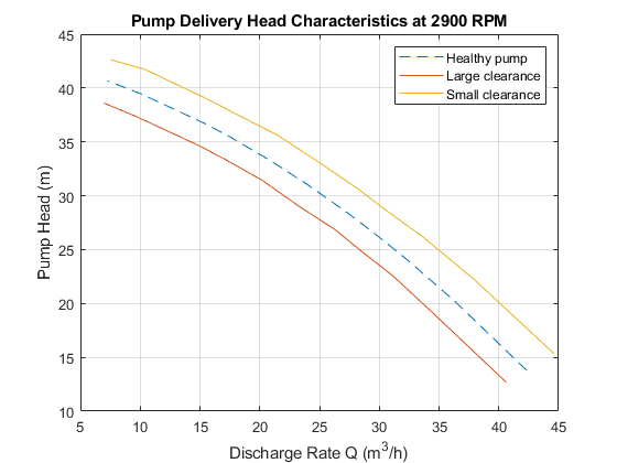
Similar changes can be seen in torque-flow characteristics and for other fault types.

For automation of fault diagnosis, you turn the observed changes to quantitative information. A reliable way to do so is to fit a parameterized curve to the head-flow characteristic data plotted above. Using the pump-pipe dynamics governing equations, and using a simplified torque relationship, the following equations are obtained:

${\mathit{h}}_{\mathrm{nn}},{\mathit{h}}_{\mathrm{nv}},{\mathit{h}}_{\mathrm{vv}},{\mathit{k}}_0,{\mathit{k}}_1,{\mathit{k}}_2$ are the parameters to be estimated. If you measure $\omega ,\mathit{Q},\mathit{H}$and ${\mathit{M}}_{\mathit{p}}$, the parameter can be estimated by linear least squares. These parameters are the features that can be used to develop a fault detection and diagnosis algorithm.

Preliminary Analysis: Comparing Parameter Values

Compute and plot the parameter values estimated for the above 3 curves. Use the measured values of $\mathit{Q},\mathit{H}$ and ${\mathit{M}}_{\mathit{p}}$ as data and $$\omega =2900RPM$$ as the nominal pump speed.

w = 2900; % RPM
% Healthy pump
[hnn_0, hnv_0, hvv_0, k0_0, k1_0, k2_0] = linearFit(0, {w, Q0, H0, M0});
% Pump with large clearance
[hnn_1, hnv_1, hvv_1, k0_1, k1_1, k2_1] = linearFit(0, {w, Q1, H1, M1});
% Pump with small clearance
[hnn_2, hnv_2, hvv_2, k0_2, k1_2, k2_2] = linearFit(0, {w, Q2, H2, M2});
X = [hnn_0 hnn_1 hnn_2; hnv_0  hnv_1  hnv_2; hvv_0  hvv_1  hvv_2]';
disp(array2table(X,'VariableNames',{'hnn','hnv','hvv'},...
    'RowNames',{'Healthy','Large Clearance', 'Small Clearance'}))

                          hnn           hnv           hvv   
                       __________    __________    _________

    Healthy            5.1164e-06    8.6148e-05     0.010421
    Large Clearance     4.849e-06     8.362e-05     0.011082
    Small Clearance    5.3677e-06    8.4764e-05    0.0094656

Y = [k0_0 k0_1 k0_2; k1_0  k1_1  k1_2; k2_0  k2_1  k2_2]';
disp(array2table(Y,'VariableNames',{'k0','k1','k2'},...
    'RowNames',{'Healthy','Large Clearance', 'Small Clearance'}))

                           k0           k1           k2    
                       __________    ________    __________

    Healthy            0.00033347    0.016535    2.8212e-07
    Large Clearance    0.00031571    0.016471    3.0285e-07
    Small Clearance    0.00034604    0.015886    2.6669e-07

The tables show that ${\mathit{h}}_{\mathrm{nn}}$ and ${\mathit{k}}_0$ values reduce when clearance gap is large while they are larger than nominal values for small clearance. On the other hand, ${\mathit{h}}_{\mathrm{vv}}$ and ${\mathit{k}}_2$ values increase for large clearance gap and decrease for small gap. The dependence of ${\mathit{h}}_{\mathrm{nv}}$ and ${\mathit{k}}_1$ on clearance gap is less clear.

Incorporating Uncertainty

The preliminary analysis showed how parameter changes can indicate fault. However, even for healthy pumps there are variations in measurements owing to the measurement noise, fluid contamination and viscosity changes and the slip-torque characteristics of the motor running the pump. These measurement variations introduce uncertainty in the parameter estimates.

Collect 5 sets of measurements from a pump operating under no-fault condition by running it at 2900 RPM for 10 discharge throttle valve positions.

url = 'https://www.mathworks.com/supportfiles/predmaint/fault-diagnosis-of-centrifugal-pumps-using-steady-state-experiments/FaultDiagnosisData.mat';
websave('FaultDiagnosisData.mat',url);
load FaultDiagnosisData HealthyEnsemble
H = cellfun(@(x)x.Head,HealthyEnsemble,'uni',0);
Q = cellfun(@(x)x.Discharge,HealthyEnsemble,'uni',0);
plot(cat(2,Q{:}),cat(2,H{:}),'k.')
title('Pump Head Characteristics Ensemble for 5 Test Runs')
xlabel('Flow rate (m^3/hed)')
ylabel('Pump head (m)')

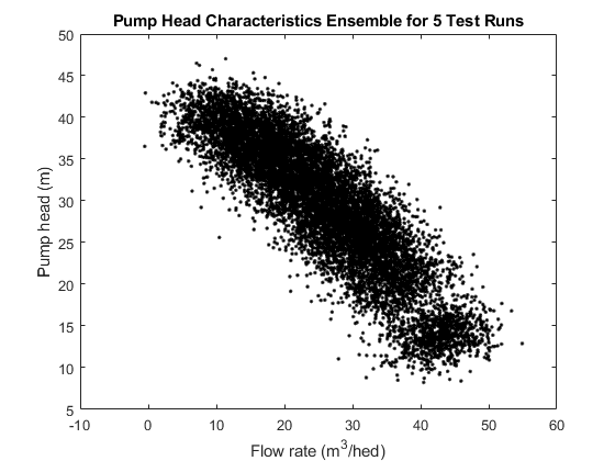
The plot shows variation in characteristics even for a healthy pump under realistic conditions. These variations have to be taken into consideration for making the fault diagnosis reliable. The next sections discuss fault detection and isolation techniques for noisy data.

Anomaly Detection

In many situations, the measurements of only the healthy machines are available. In that case, a statistical description of the healthy state, encapsulated by mean value and covariance of the parameter vector, can be created using available measurements. The measurements of the test pump can be compared against the nominal statistics to test whether it is plausible that the test pump is a healthy pump. A faulty pump is expected to detected as an anomaly in a view of detection features.

Estimate mean and covariance of pump head and torque parameters.

load FaultDiagnosisData HealthyEnsemble
[HealthyTheta1, HealthyTheta2] = linearFit(1, HealthyEnsemble);
meanTheta1 = mean(HealthyTheta1,1);
meanTheta2 = mean(HealthyTheta2,1);
covTheta1  = cov(HealthyTheta1);
covTheta2  = cov(HealthyTheta2);

Visualize the parameter uncertainty as 74% confidence regions, which corresponds to 2 standard deviations ($$\sqrt{chi2inv(0.74,3)}\approx 2$$). See helper function helperPlotConfidenceEllipsoid for details.

% Confidence ellipsoid for pump head parameters
f = figure;
f.Position(3) = f.Position(3)*2;
subplot(121)
helperPlotConfidenceEllipsoid(meanTheta1,covTheta1,2,0.6);   
xlabel('hnn')
ylabel('hnv')
zlabel('hvv')
title('2-sd Confidence Ellipsoid for Pump Head Parameters')
hold on

% Confidence ellipsoid for pump torque parameters
subplot(122)
helperPlotConfidenceEllipsoid(meanTheta2,covTheta2,2,0.6); 
xlabel('k0')
ylabel('k1')
zlabel('k2')
title('2-sd Confidence Ellipsoid for Pump Torque Parameters')
hold on

The grey ellipsoids show confidence regions of healthy pump parameters. Load unlabeled test data for comparison against the healthy region.

load FaultDiagnosisData TestEnsemble

TestEnsemble contains a set of pump speed, torque, head and flow rate measurements at various valve positions. All measurements contain clearance gap fault of different magnitudes.

% Test data preview
disp(TestEnsemble{1}(1:5,:)) % first 5 measurement rows from the first ensemble member

      Time       Run    ValvePosition    Speed      Head     Discharge    Torque 
    _________    ___    _____________    ______    ______    _________    _______

    180 sec       1          10          3034.6    12.367     35.339      0.35288
    180.1 sec     1          10          2922.1    9.6762     36.556       4.6953
    180.2 sec     1          10          2636.1    11.168     36.835       9.8898
    180.3 sec     1          10          2717.4    10.562      40.22      -12.598
    180.4 sec     1          10          3183.7     10.55     40.553       14.672

Compute test parameters. See helper function linearFit.

% TestTheta1: pump head parameters
% TestTheta2: pump torque parameters
[TestTheta1,TestTheta2] = linearFit(1, TestEnsemble);
subplot(121)
plot3(TestTheta1(:,1),TestTheta1(:,2),TestTheta1(:,3),'g*')
view([-42.7 10])
subplot(122)
plot3(TestTheta2(:,1),TestTheta2(:,2),TestTheta2(:,3),'g*')
view([-28.3 18])

Each green star marker is contributed by one test pump. The markers that are outside the confidence bounds can be treated as outliers while those inside are either from a healthy pump or escaped detection. Note that a marker from a particular pump may be marked as anomalous in the pump head view but not in the pump torque view. This could be owing to different sources of faults being detected by these views, or the underlying reliability of pressure and torque measurements.

Quantifying Anomaly Detection Using Confidence Regions

In this section a way of utilizing the confidence region information for detection and assessing severity of faults is discussed. The technique is to compute the "distance" of a test sample from the mean or median of the healthy region distribution. The distance must be relative to the normal "spread" of the healthy parameter data represented by its covariance. The function MAHAL computes the Mahalanobis distance of test samples from the distribution of a reference sample set (the healthy pump parameter set here):

ParDist1 = mahal(TestTheta1, HealthyTheta1);  % for pump head parameters

If you assume 74% confidence bound (2 standard deviations) as acceptable variation for healthy data, any values in ParDist1 that are greater than 2^2 = 4 should be tagged as anomalous and hence indicative of faulty behavior.

Add the distance values to the plot. The red lines mark the anomalous test samples. See helper function helperAddDistanceLines.

Threshold = 2;
disp(table((1:length(ParDist1))',ParDist1, ParDist1>Threshold^2,...
    'VariableNames',{'PumpNumber','SampleDistance','Anomalous'}))

    PumpNumber    SampleDistance    Anomalous
    __________    ______________    _________

         1            58.874          true   
         2            24.051          true   
         3             6.281          true   
         4            3.7179          false  
         5             13.58          true   
         6            3.0723          false  
         7            2.0958          false  
         8            4.7127          true   
         9            26.829          true   
        10           0.74682          false  

helperAddDistanceLines(1, ParDist1, meanTheta1, TestTheta1, Threshold);

Similarly for pump torque:

ParDist2 = mahal(TestTheta2, HealthyTheta2);  % for pump torque parameters
disp(table((1:length(ParDist2))',ParDist2, ParDist2>Threshold^2,...
    'VariableNames',{'PumpNumber','SampleDistance','Anomalous'}))

    PumpNumber    SampleDistance    Anomalous
    __________    ______________    _________

         1            9.1381          true   
         2            5.4249          true   
         3            3.0565          false  
         4             3.775          false  
         5           0.77961          false  
         6            7.5508          true   
         7            3.3368          false  
         8           0.74834          false  
         9            3.6478          false  
        10            1.0241          false  

helperAddDistanceLines(2, ParDist2, meanTheta2, TestTheta2, Threshold);
view([8.1 17.2])

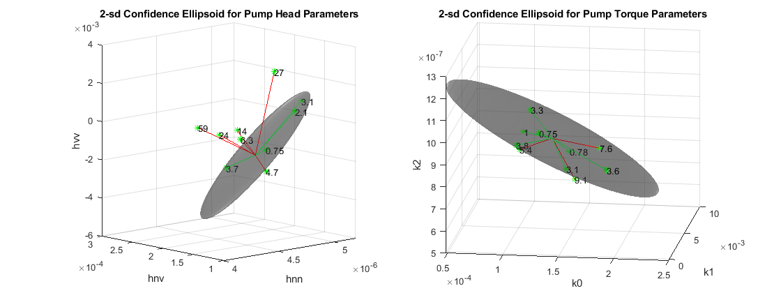
The plots now not only show detection of the anomalous samples but also quantify their severity.

Quantifying Anomaly Detection Using One-Class Classifier

Another effective technique to flag anomalies is to build a one-class classifier for the healthy parameter dataset. Train an SVM classifier using the healthy pump parameter data. Since there are no fault labels utilized, treat all samples as coming from the same (healthy) class. Since changes in parameters ${\mathit{h}}_{\mathrm{nn}}$ and ${\mathit{h}}_{\mathrm{vv}}$ are most indicative of potential faults, use only these parameters for training the SVM classifier.

nc = size(HealthyTheta1,1);
rng(2)  % for reproducibility
SVMOneClass1 = fitcsvm(HealthyTheta1(:,[1 3]),ones(nc,1),...
    'KernelScale','auto',...
    'Standardize',true,...
    'OutlierFraction',0.0455);

Plot the test observations and the decision boundary. Flag the support vectors and potential outliers. See helper function helperPlotSVM.

figure
helperPlotSVM(SVMOneClass1,TestTheta1(:,[1 3]))
title('SVM Anomaly Detection for Pump Head Parameters')
xlabel('hnn')
ylabel('hvv')

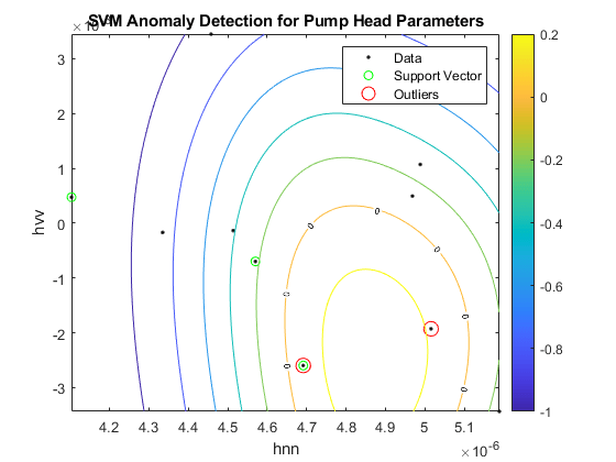
The boundary separating the outliers from the rest of the data occurs where the contour value is 0; this is the level curve marked with "0" in the plot. The outliers are marked with red circles. A similar analysis can be performed for torque parameters.

SVMOneClass2 = fitcsvm(HealthyTheta2(:,[1 3]),ones(nc,1),...
    'KernelScale','auto',...
    'Standardize',true,...
    'OutlierFraction',0.0455);
figure
helperPlotSVM(SVMOneClass2,TestTheta2(:,[1 3]))
title('SVM Anomaly Detection for Torque Parameters')
xlabel('k0')
ylabel('k2')

A similar analysis can be carried out for detecting other kinds of faults such as wear or deposits at impeller outlet as discussed next in the context of fault isolation.

Fault Isolation Using Steady-State Parameters as Features

If the information on the type of fault(s) in the test system is available, it can be used to create algorithms that not only detect faults but also indicate their type.

A. Distinguishing Clearance Gap Faults by Likelihood Ratio Tests

Changes in clearance gap can be split into two types - smaller than expected gap (yellow line in the pump head characteristic plot) and larger than expected gap (red line). Load pump test data sets containing clearance gap faults where the nature of fault (large or small) is known in advance. Use these fault labels to perform 3-way classification among the following modes:

url = 'https://www.mathworks.com/supportfiles/predmaint/fault-diagnosis-of-centrifugal-pumps-using-steady-state-experiments/LabeledGapClearanceData.mat';
websave('LabeledGapClearanceData.mat',url);
load LabeledGapClearanceData HealthyEnsemble LargeGapEnsemble SmallGapEnsemble

The ensembles contain data from 50 independent experiments. Fit steady-state linear models as before to parameterize the pump head and torque data.

[HealthyTheta1, HealthyTheta2] = linearFit(1,HealthyEnsemble);
[LargeTheta1, LargeTheta2]     = linearFit(1,LargeGapEnsemble);
[SmallTheta1, SmallTheta2]     = linearFit(1,SmallGapEnsemble);

Plot the parameter histograms to check if there is separability among the 3 modes. The function histfit is used to plot the histograms and the corresponding fitted normal distribution curves. See helper function helperPlotHistogram.

Pump head parameters:

helperPlotHistogram(HealthyTheta1, LargeTheta1, SmallTheta1, {'hnn','hnv','hvv'})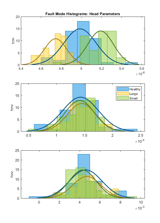

The histogram shows that ${\mathit{h}}_{\mathrm{nn}}$ offers good separability among the three modes but ${\mathit{h}}_{\mathrm{nv}},{\mathit{h}}_{\mathrm{vv}}$ parameters have overlapping probability distribution functions (PDFs).

Pump torque parameters:

helperPlotHistogram(HealthyTheta2, LargeTheta2, SmallTheta2, {'k0','k1','k2'})

For the Torque parameters, the individual separability is not very good. There is still some variation in mean and variances that can be exploited by a trained 3-mode classifier. If the PDFs show good separation in mean or variance, you can design likelihood ratio tests to quickly assign a test dataset to the most likely mode. This is shown next for the pump head parameters.

Let:

Consider the available parameter sets as test samples for mode prediction. Assign the predicted mode as belonging to one for which the joint PDF has the highest value (Hypothesis ${{\rm H}}_0$ is selected over ${{\rm H}}_1$ if $\mathit{p}\left({\mathit{H}}_0\right)>\mathit{p}\left({\mathit{H}}_1\right)$). Then plot the results comparing the true and predicted modes in a confusion matrix. Function mvnpdf is used for computing the PDF value and the functions confusionmatrix and heatmap are used for confusion matrix visualization. See helper function pumpModeLikelihoodTest.

% Pump head confusion matrix
figure
pumpModeLikelihoodTest(HealthyTheta1, LargeTheta1, SmallTheta1)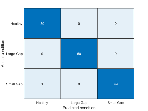

The confusion plot shows perfect separation between the three modes, which is not surprising given the clear separation among the histograms for ${\mathit{h}}_{\mathrm{nn}}$ parameters.

% Pump torque confusion matrix
pumpModeLikelihoodTest(HealthyTheta2, LargeTheta2, SmallTheta2)

The results are slightly worse for the torque parameters. Still, the success rate is quite high (97%) even though the PDFs of the three modes overlapped significantly. This is because the PDF value calculation is affected both by the location (mean) as well as the amplitude (variance).

B. Multi-Class Classification of Fault Modes Using Tree Bagging

In this section, another classification technique is discussed that is more suitable when classification among a larger number of modes is required. Consider the following fault modes of operation of the pump:

The classification problem is harder because there are only three parameters computed and you need to distinguish among 7 modes of operation. Thus, not only you have to compare the estimated parameters for each fault mode to the healthy mode, but also to each other - both the direction (increase or reduction in value) and magnitude (10% change vs. 70% change) of the parameter change must be taken into consideration.

Here the use of TreeBagger classifier for this problem is shown. Tree Bagger is an ensemble learning technique that uses bootstrap aggregation (bagging) of features to create decision trees that classify labeled data. 50 labeled data sets are collected for the 7 modes of operation. Estimate pump head parameters for each dataset and train the classifier using a subset of the parameter estimates from each mode.

url = 'https://www.mathworks.com/supportfiles/predmaint/fault-diagnosis-of-centrifugal-pumps-using-steady-state-experiments/MultipleFaultsData.mat';
websave('MultipleFaultsData.mat',url);
load MultipleFaultsData
% Compute pump head parameters
HealthyTheta = linearFit(1, HealthyEnsemble);
Fault1Theta  = linearFit(1, Fault1Ensemble);
Fault2Theta  = linearFit(1, Fault2Ensemble);
Fault3Theta  = linearFit(1, Fault3Ensemble);
Fault4Theta  = linearFit(1, Fault4Ensemble);
Fault5Theta  = linearFit(1, Fault5Ensemble);
Fault6Theta  = linearFit(1, Fault6Ensemble);

% Generate labels for each mode of operation
Label = {'Healthy','ClearanceGapWear','ImpellerOutletDeposit',...
    'ImpellerInletDeposit','AbrasiveWear','BrokenBlade','Cavitation'};
VarNames = {'hnn','hnv','hvv','Condition'};
% Assemble results in a table with parameters and corresponding labels 
N = 50; 
T0 = [array2table(HealthyTheta),repmat(Label(1),[N,1])];
T0.Properties.VariableNames = VarNames;
T1 = [array2table(Fault1Theta), repmat(Label(2),[N,1])];
T1.Properties.VariableNames = VarNames;
T2 = [array2table(Fault2Theta), repmat(Label(3),[N,1])];
T2.Properties.VariableNames = VarNames;
T3 = [array2table(Fault3Theta), repmat(Label(4),[N,1])];
T3.Properties.VariableNames = VarNames;
T4 = [array2table(Fault4Theta), repmat(Label(5),[N,1])];
T4.Properties.VariableNames = VarNames;
T5 = [array2table(Fault5Theta), repmat(Label(6),[N,1])];
T5.Properties.VariableNames = VarNames;
T6 = [array2table(Fault6Theta), repmat(Label(7),[N,1])];
T6.Properties.VariableNames = VarNames;

% Stack all data
% Use 30 out of 50 datasets for model creation
TrainingData = [T0(1:30,:);T1(1:30,:);T2(1:30,:);T3(1:30,:);T4(1:30,:);T5(1:30,:);T6(1:30,:)];

% Create an ensemble Mdl of 20 decision trees for predicting the 
% labels using the parameter values
rng(3) % for reproducibility
Mdl = TreeBagger(20, TrainingData, 'Condition',...
   'OOBPrediction','on',...
   'OOBPredictorImportance','on')

Mdl = 
  TreeBagger
Ensemble with 20 bagged decision trees:
                    Training X:              [210x3]
                    Training Y:              [210x1]
                        Method:       classification
                 NumPredictors:                    3
         NumPredictorsToSample:                    2
                   MinLeafSize:                    1
                 InBagFraction:                    1
         SampleWithReplacement:                    1
          ComputeOOBPrediction:                    1
 ComputeOOBPredictorImportance:                    1
                     Proximity:                   []
                    ClassNames:  'AbrasiveWear'   'BrokenBlade'    'Cavitation' 'ClearanceGapWear'       'Healthy' 'ImpellerInletDeposit' 'ImpellerOutletDeposit'

  Properties, Methods

The performance of the TreeBagger model can be computed by studying its misclassification probability for out-of-bag observations as a function of number of decision trees.

% Compute out of bag error
figure
plot(oobError(Mdl))
xlabel('Number of trees')
ylabel('Misclassification probability')

Finally, compute prediction performance of the model on test samples that were never used for growing the decision trees.

ValidationData = [T0(31:50,:);T1(31:50,:);T2(31:50,:);T3(31:50,:);T4(31:50,:);T5(31:50,:);T6(31:50,:)];
PredictedClass = predict(Mdl,ValidationData);
E = zeros(1,7);
% Healthy data misclassification
E(1) = sum(~strcmp(PredictedClass(1:20), Label{1}));
% Clearance gap fault misclassification
E(2) = sum(~strcmp(PredictedClass(21:40), Label{2}));
% Impeller outlet deposit fault misclassification
E(3) = sum(~strcmp(PredictedClass(41:60), Label{3}));
% Impeller inlet deposit fault misclassification
E(4) = sum(~strcmp(PredictedClass(61:80), Label{4}));
% Abrasive wear fault misclassification
E(5) = sum(~strcmp(PredictedClass(81:100), Label{5}));
% Broken blade fault misclassification
E(6) = sum(~strcmp(PredictedClass(101:120), Label{6}));
% Cavitation fault misclassification
E(7) = sum(~strcmp(PredictedClass(121:140), Label{7}));
figure
bar(E/20*100)
xticklabels(Label)
set(gca,'XTickLabelRotation',45)
ylabel('Misclassification (%)')

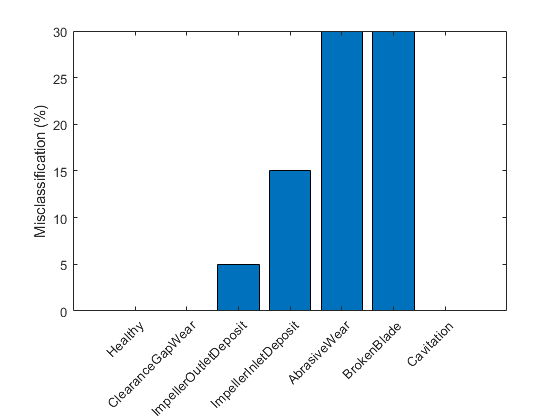
The plot shows that the abrasive wear and broken blade faults are misclassified for 30% of the validation samples. A closer look at the predicted labels shows that in the misclassified cases, the 'AbrasiveWear' and 'BrokenBlade' labels get intermixed between each other only. This suggests that the symptoms for these fault categories are not sufficiently distinguishable for this classifier.

Summary

A well designed fault diagnosis strategy can save operating costs by minimizing service downtime and component replacement costs. The strategy benefits from a good knowledge about the operating machine's dynamics which is used in combination with sensor measurements to detect and isolate different kinds of faults.

This example discussed a parametric approach for fault detection and isolation based on steady-state experiments. This approach requires careful modeling of the system dynamics and using the parameters (or transformations thereof) as features for designing fault diagnosis algorithms. The parameters were used for training anomaly detectors, performing likelihood ratio tests and for training of multi-class classifiers.

How to make use of classification techniques in real-life testing of pumps

A summary of the fault diagnosis workflow follows.

For a fault diagnosis approach based on residual analysis, see the Fault Diagnosis of Centrifugal Pumps Using Residual Analysis example.

References

Supporting Functions

Linear fit to pump parameters.

function varargout = linearFit(Form, Data)
%linearFit Linear least squares solution for Pump Head and Torque parameters.
%
% If Form==0, accept separate inputs and return separate outputs. For one experiment only.
% If Form==1, accept an ensemble and return compact parameter vectors. For several experiments (ensemble).
if Form==0
   w = Data{1};
   Q = Data{2};
   H = Data{3};
   M = Data{4};
   n = length(Q);
   if isscalar(w), w = w*ones(n,1); end
   Q = Q(:); H = H(:); M = M(:);
   Predictor = [w.^2, w.*Q, Q.^2];
   Theta1 = Predictor\H;
   hnn =  Theta1(1);
   hnv = -Theta1(2);
   hvv = -Theta1(3);
   Theta2 = Predictor\M;
   k0 =  Theta2(2);
   k1 = -Theta2(3);
   k2 =  Theta2(1);
   varargout = {hnn, hnv, hvv, k0, k1, k2};
else
   H = cellfun(@(x)x.Head,Data,'uni',0);
   Q = cellfun(@(x)x.Discharge,Data,'uni',0);
   M = cellfun(@(x)x.Torque,Data,'uni',0);
   W = cellfun(@(x)x.Speed,Data,'uni',0);
   N = numel(H);

   Theta1 = zeros(3,N);
   Theta2 = zeros(3,N);
   
   for kexp = 1:N
      Predictor = [W{kexp}.^2, W{kexp}.*Q{kexp}, Q{kexp}.^2];
      X1 = Predictor\H{kexp};
      hnn =  X1(1);
      hnv = -X1(2);
      hvv = -X1(3);
      X2 = Predictor\M{kexp};
      k0 =  X2(2);
      k1 = -X2(3);
      k2 =  X2(1);
      
      Theta1(:,kexp) = [hnn; hnv; hvv];
      Theta2(:,kexp) = [k0; k1; k2];
   end
   varargout = {Theta1', Theta2'};
end
end

Membership likelihood test.

function pumpModeLikelihoodTest(HealthyTheta, LargeTheta, SmallTheta)
%pumpModeLikelihoodTest Generate predictions based on PDF values and plot confusion matrix.

m1 = mean(HealthyTheta);
c1 = cov(HealthyTheta);
m2 = mean(LargeTheta);
c2 = cov(LargeTheta);
m3 = mean(SmallTheta);
c3 = cov(SmallTheta);

N = size(HealthyTheta,1);

% True classes
% 1: Healthy: group label is 1.
X1t = ones(N,1);
% 2: Large gap: group label is 2.
X2t = 2*ones(N,1);
% 3: Small gap: group label is 3.
X3t = 3*ones(N,1);

% Compute predicted classes as those for which the joint PDF has the maximum value.
X1 = zeros(N,3); 
X2 = zeros(N,3); 
X3 = zeros(N,3); 
for ct = 1:N
   % Membership probability density for healthy parameter sample
   HealthySample  = HealthyTheta(ct,:);
   x1 = mvnpdf(HealthySample, m1, c1);
   x2 = mvnpdf(HealthySample, m2, c2);
   x3 = mvnpdf(HealthySample, m3, c3);
   X1(ct,:) = [x1 x2 x3];
   
   % Membership probability density for large gap pump parameter
   LargeSample  = LargeTheta(ct,:);
   x1 = mvnpdf(LargeSample, m1, c1);
   x2 = mvnpdf(LargeSample, m2, c2);
   x3 = mvnpdf(LargeSample, m3, c3);
   X2(ct,:) = [x1 x2 x3];
   
   % Membership probability density for small gap pump parameter
   SmallSample  = SmallTheta(ct,:);
   x1 = mvnpdf(SmallSample, m1, c1);
   x2 = mvnpdf(SmallSample, m2, c2);
   x3 = mvnpdf(SmallSample, m3, c3);
   X3(ct,:) = [x1 x2 x3];
end

[~,PredictedGroup] = max([X1;X2;X3],[],2);
TrueGroup = [X1t; X2t; X3t];
C = confusionmat(TrueGroup,PredictedGroup);
heatmap(C, ...
    'YLabel', 'Actual condition', ...
    'YDisplayLabels', {'Healthy','Large Gap','Small Gap'}, ...
    'XLabel', 'Predicted condition', ...
    'XDisplayLabels', {'Healthy','Large Gap','Small Gap'}, ...
    'ColorbarVisible','off');
end

References

Isermann, Rolf, Fault-Diagnosis Applications. Model-Based Condition Monitoring: Actuators, Drives, Machinery, Plants, Sensors, and Fault-tolerant System, Edition 1, Springer-Verlag Berlin Heidelberg, 2011.